Cross-validating mixed-effects models

The fundamental analogy for cross-validation is to the collection of new data. That is, predicting the response in each fold from the model fit to data in the other folds is like using the model fit to all of the data to predict the response for new cases from the values of the predictors for those new cases. As we explained in the introductory vignette on cross-validating regression models, the application of this idea to independently sampled cases is straightforward—simply partition the data into random folds of equal size and leave each fold out in turn, or, in the case of LOO CV, simply omit each case in turn.

In contrast, mixed-effects models are fit to dependent data, in which cases as clustered, such as hierarchical data, where the clusters comprise higher-level units (e.g., students clustered in schools), or longitudinal data, where the clusters are individuals and the cases repeated observations on the individuals over time.¹

We can think of two approaches to applying cross-validation to clustered data:²

Treat CV as analogous to predicting the response for one or more cases in a newly observed cluster. In this instance, the folds comprise one or more whole clusters; we refit the model with all of the cases in clusters in the current fold removed; and then we predict the response for the cases in clusters in the current fold. These predictions are based only on fixed effects because the random effects for the omitted clusters are presumably unknown, as they would be for data on cases in newly observed clusters.
Treat CV as analogous to predicting the response for a newly observed case in an existing cluster. In this instance, the folds comprise one or more individual cases, and the predictions can use both the fixed and random effects.

Example: The High-School and Beyond data

Following their use by Raudenbush & Bryk (2002), data from the 1982 High School and Beyond (HSB) survey have become a staple of the literature on mixed-effects models. The HSB data are used by Fox & Weisberg (2019, sec. 7.2.2) to illustrate the application of linear mixed models to hierarchical data, and we’ll closely follow their example here.

The HSB data are included in the MathAchieve and MathAchSchool data sets in the nlme package (Pinheiro & Bates, 2000). MathAchieve includes individual-level data on 7185 students in 160 high schools, and MathAchSchool includes school-level data:

data("MathAchieve", package = "nlme")
dim(MathAchieve)
#> [1] 7185    6
head(MathAchieve, 3)
#> Grouped Data: MathAch ~ SES | School
#>   School Minority    Sex    SES MathAch MEANSES
#> 1   1224       No Female -1.528   5.876  -0.428
#> 2   1224       No Female -0.588  19.708  -0.428
#> 3   1224       No   Male -0.528  20.349  -0.428
tail(MathAchieve, 3)
#> Grouped Data: MathAch ~ SES | School
#>      School Minority    Sex    SES MathAch MEANSES
#> 7183   9586       No Female  1.332  19.641   0.627
#> 7184   9586       No Female -0.008  16.241   0.627
#> 7185   9586       No Female  0.792  22.733   0.627

data("MathAchSchool", package = "nlme")
dim(MathAchSchool)
#> [1] 160   7
head(MathAchSchool, 2)
#>      School Size Sector PRACAD DISCLIM HIMINTY MEANSES
#> 1224   1224  842 Public   0.35   1.597       0  -0.428
#> 1288   1288 1855 Public   0.27   0.174       0   0.128
tail(MathAchSchool, 2)
#>      School Size   Sector PRACAD DISCLIM HIMINTY MEANSES
#> 9550   9550 1532   Public   0.45   0.791       0   0.059
#> 9586   9586  262 Catholic   1.00  -2.416       0   0.627

The first few students are in school number 1224 and the last few in school 9586.

We’ll use only the School, SES (students’ socioeconomic status), and MathAch (their score on a standardized math-achievement test) variables in the MathAchieve data set, and Sector ("Catholic" or "Public") in the MathAchSchool data set.

Some data-management is required before fitting a mixed-effects model to the HSB data, for which we use the dplyr package (Wickham, François, Henry, Müller, & Vaughan, 2023):

library("dplyr")
MathAchieve %>% group_by(School) %>%
  summarize(mean.ses = mean(SES)) -> Temp
Temp <- merge(MathAchSchool, Temp, by = "School")
HSB <- merge(Temp[, c("School", "Sector", "mean.ses")],
             MathAchieve[, c("School", "SES", "MathAch")], by = "School")
names(HSB) <- tolower(names(HSB))

HSB$cses <- with(HSB, ses - mean.ses)

In the process, we created two new school-level variables: meanses, which is the average SES for students in each school; and cses, which is school-average SES centered at its mean. For details, see Fox & Weisberg (2019, sec. 7.2.2).

Still following Fox and Weisberg, we proceed to use the lmer() function in the lme4 package (Bates, Mächler, Bolker, & Walker, 2015) to fit a mixed model for math achievement to the HSB data:

library("lme4")
hsb.lmer <- lmer(mathach ~ mean.ses * cses + sector * cses
                 + (cses | school), data = HSB)
summary(hsb.lmer, correlation = FALSE)
#> Linear mixed model fit by REML ['lmerMod']
#> Formula: mathach ~ mean.ses * cses + sector * cses + (cses | school)
#>    Data: HSB
#> 
#> REML criterion at convergence: 46504
#> 
#> Scaled residuals: 
#>    Min     1Q Median     3Q    Max 
#> -3.159 -0.723  0.017  0.754  2.958 
#> 
#> Random effects:
#>  Groups   Name        Variance Std.Dev. Corr
#>  school   (Intercept)  2.380   1.543        
#>           cses         0.101   0.318    0.39
#>  Residual             36.721   6.060        
#> Number of obs: 7185, groups:  school, 160
#> 
#> Fixed effects:
#>                     Estimate Std. Error t value
#> (Intercept)           12.128      0.199   60.86
#> mean.ses               5.333      0.369   14.45
#> cses                   2.945      0.156   18.93
#> sectorCatholic         1.227      0.306    4.00
#> mean.ses:cses          1.039      0.299    3.48
#> cses:sectorCatholic   -1.643      0.240   -6.85

We can then cross-validate at the cluster (i.e., school) level,

library("cv")

cv(hsb.lmer,
   k = 10,
   clusterVariables = "school",
   seed = 5240)
#> R RNG seed set to 5240
#> 10-Fold Cross Validation based on 160 {school} clusters
#> criterion: mse
#> cross-validation criterion = 39.157
#> bias-adjusted cross-validation criterion = 39.148
#> 95% CI for bias-adjusted CV criterion = (38.066, 40.231)
#> full-sample criterion = 39.006

or at the case (i.e., student) level,

cv(hsb.lmer, seed = 1575)
#> R RNG seed set to 1575
#> Warning in checkConv(attr(opt, "derivs"), opt$par, ctrl = control$checkConv, :
#> Model failed to converge with max|grad| = 0.00587207 (tol = 0.002, component 1)
#> boundary (singular) fit: see help('isSingular')
#> 10-Fold Cross Validation
#> criterion: mse
#> cross-validation criterion = 37.445
#> bias-adjusted cross-validation criterion = 37.338
#> 95% CI for bias-adjusted CV criterion = (36.288, 38.388)
#> full-sample criterion = 36.068

For cluster-level CV, the clusterVariables argument tells cv() how the clusters are defined. Were there more than one clustering variable, say classes within schools, these would be provided as a character vector of variable names: clusterVariables = c("school", "class"). For cluster-level CV, the default is k = "loo", that is, leave one cluster out at a time; we instead specify k = 10 folds of clusters, each fold therefore comprising $160/10 = 16$ schools.

If the clusterVariables argument is omitted, then case-level CV is employed, with k = 10 folds as the default, here each with $7185/10 \approx 719$ students. Notice that one of the 10 models refit with a fold removed failed to converge. Convergence problems are common in mixed-effects modeling. The apparent issue here is that an estimated variance component is close to or equal to 0, which is at a boundary of the parameter space. That shouldn’t disqualify the fitted model for the kind of prediction required for cross-validation.

There is also a cv() method for linear mixed models fit by the lme() function in the nlme package, and the arguments for cv() in this case are the same as for a model fit by lmer() or glmer(). We illustrate with the mixed model fit to the HSB data:

library("nlme")
hsb.lme <- lme(
  mathach ~ mean.ses * cses + sector * cses,
  random = ~ cses | school,
  data = HSB,
  control = list(opt = "optim")
)
summary(hsb.lme)
#> Linear mixed-effects model fit by REML
#>   Data: HSB 
#>     AIC   BIC logLik
#>   46525 46594 -23252
#> 
#> Random effects:
#>  Formula: ~cses | school
#>  Structure: General positive-definite, Log-Cholesky parametrization
#>             StdDev   Corr  
#> (Intercept) 1.541177 (Intr)
#> cses        0.018174 0.006 
#> Residual    6.063492       
#> 
#> Fixed effects:  mathach ~ mean.ses * cses + sector * cses 
#>                       Value Std.Error   DF t-value p-value
#> (Intercept)         12.1282   0.19920 7022  60.886   0e+00
#> mean.ses             5.3367   0.36898  157  14.463   0e+00
#> cses                 2.9421   0.15122 7022  19.456   0e+00
#> sectorCatholic       1.2245   0.30611  157   4.000   1e-04
#> mean.ses:cses        1.0444   0.29107 7022   3.588   3e-04
#> cses:sectorCatholic -1.6421   0.23312 7022  -7.044   0e+00
#>  Correlation: 
#>                     (Intr) men.ss cses   sctrCt mn.ss:
#> mean.ses             0.256                            
#> cses                 0.000  0.000                     
#> sectorCatholic      -0.699 -0.356  0.000              
#> mean.ses:cses        0.000  0.000  0.295  0.000       
#> cses:sectorCatholic  0.000  0.000 -0.696  0.000 -0.351
#> 
#> Standardized Within-Group Residuals:
#>       Min        Q1       Med        Q3       Max 
#> -3.170106 -0.724877  0.014892  0.754263  2.965498 
#> 
#> Number of Observations: 7185
#> Number of Groups: 160

cv(hsb.lme,
   k = 10,
   clusterVariables = "school",
   seed = 5240)
#> R RNG seed set to 5240
#> 10-Fold Cross Validation based on 160 {school} clusters
#> criterion: mse
#> cross-validation criterion = 39.157
#> bias-adjusted cross-validation criterion = 39.149
#> 95% CI for bias-adjusted CV criterion = (38.066, 40.232)
#> full-sample criterion = 39.006

cv(hsb.lme, seed = 1575)
#> R RNG seed set to 1575
#> 10-Fold Cross Validation
#> criterion: mse
#> cross-validation criterion = 37.442
#> bias-adjusted cross-validation criterion = 37.402
#> 95% CI for bias-adjusted CV criterion = (36.351, 38.453)
#> full-sample criterion = 36.147

We used the same random-number generator seeds as in the previous example cross-validating the model fit by lmer(), and so the same folds are employed in both cases.³ The estimated covariance components and fixed effects in the summary output differ slightly between the lmer() and lme() solutions, although both functions seek to maximize the REML criterion. This is, of course, to be expected when different algorithms are used for numerical optimization. To the precision reported, the cluster-level CV results for the lmer() and lme() models are identical, while the case-level CV results are very similar but not identical.

Example: Contrasting cluster-based and case-based CV

We introduce four artificial data sets that exemplify aspects of cross-validation particular to hierarchical models. Using these data sets, we show that model comparisons employing cluster-based and those employing case-based cross-validation may not agree on a “best” model. Furthermore, commonly used measures of fit, such as mean-squared error, do not necessarily become smaller as models become larger, even when the models are nested, and even when the measure of fit is computed for the whole data set.

The four datasets differ in the relative magnitude of between-cluster variance compared with within-cluster variance. They serve to illustrate how fitting mixed models, and, consequently, the cross-validation of mixed models, is sensitive to relative variance, which determines the degree of shrinkage of within-cluster estimates of effects towards between-cluster estimates.

For these analyses, we will use the glmmTMB() function in the glmmTMB package (Brooks et al., 2017) because, in our experience, it is more likely to converge than functions in the nlme and the lme4 packages for models with low between-cluster variance.

Consider a researcher studying the effect of the dosage of a drug on the severity of symptoms for a hypothetical disease. The researcher has longitudinal data on 20 patients, each of whom was observed on five occasions in which patients received different dosages of the drug. The data are observational, with dosages prescribed by the patients’ physicians, so that patients who were more severely affected by the disease received higher dosages of the drug.

Our four contrived data sets (see below) illustrate possible results for data obtained in such a scenario. The relative configuration of dosages x and symptoms y are identical within patients in each of the four datasets. Within patients, higher dosages are generally associated with a reduction in symptoms.

Between patients, however, higher dosages are associated with higher levels of symptoms. A plausible mechanism is a reversal of causality: Within patients, higher dosages alleviate symptoms, but between patients higher morbidity causes the prescription of higher dosages.

The four data sets differ in the between-patient variance of patient centroids from a common between-patients regression line. The data sets exhibit a progression from low to high variance around the common regression line.

We start by generating a data set to serve as a common template for the four sample data sets. We then apply different multipliers to the between-patient variation using parameters consistent with the description above to highlight the issues that arise in cross-validating mixed-effects models:⁴


# Parameters:

Nb <- 20     # number of patients
Nw <- 5      # number of occasions for each patient

Bb <- 1.0    # between-patient regression coefficient on patient means
Bw <- -0.5   # within-patient effect of x

SD_between <- c(0, 5, 6, 8)               # SD between patients
SD_within <- rep(2.5, length(SD_between)) # SD within patients

Nv <- length(SD_within)       # number of variance profiles
SD_ratio <- paste0('SD ratio = ', SD_between,' / ',SD_within)
SD_ratio <- factor(SD_ratio, levels = SD_ratio)

set.seed(833885) 

Data_template <- expand.grid(patient = 1:Nb, obs = 1:Nw) |>
  within({
    xw <- seq(-2, 2, length.out = Nw)[obs]
    x <- patient + xw
    xm  <- ave(x, patient)   # within-patient mean

    # Scaled random error within each SD_ratio_i group

    re_std <- scale(resid(lm(rnorm(Nb*Nw) ~ x)))
    re_between <- ave(re_std, patient)
    re_within <- re_std - re_between
    re_between <- scale(re_between)/sqrt(Nw)
    re_within <- scale(re_within)
  })

Data <- do.call(
  rbind,
  lapply(
    1:Nv,
    function(i) {
      cbind(Data_template, SD_ratio_i = i)
    }
  )
)

Data <- within(
  Data,
  {
    SD_within_ <- SD_within[SD_ratio_i]
    SD_between_ <- SD_between[SD_ratio_i]
    SD_ratio <- SD_ratio[SD_ratio_i]
    y <- 10 +
      Bb * xm +                  # contextual effect
      Bw * (x - xm) +            # within-patient effect
      SD_within_ * re_within +   # within patient random effect
      SD_between_ * re_between   # adjustment to between patient random effect
  }
)

Here is a scatterplot of the data sets showing estimated 50% concentration ellipses for each cluster:⁵

library("lattice")
library("latticeExtra")
plot <- xyplot(y ~ x | SD_ratio, data = Data, group = patient,
           layout = c(Nv, 1),
           par.settings = list(superpose.symbol = list(pch = 1, cex = 0.7))) +
      layer(panel.ellipse(..., center.pch = 16, center.cex = 1.5,  
                          level = 0.5),
            panel.abline(a = 10, b = 1))
plot # display graph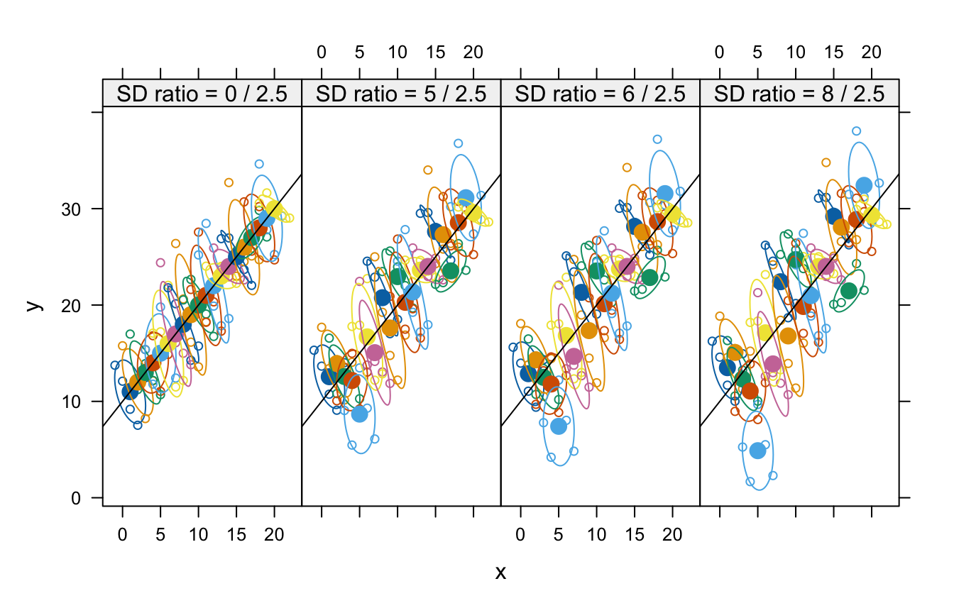

Data sets showing identical within-patient configurations with increasing between-patient variance. The labels above each panel show the between-patient SD/within-patient SD. The ellipses are estimated 50% concentration ellipses for each patient. The population between-patient regression line, $E(y) = 10 + x$ , is shown in each panel.

The population from which these datasets is generated has a between-patient effect of dosage of 1 and a within-patient effect of $-0.5$ . The researcher may attempt to obtain an estimate of the within-patient effect of dosage through the use of mixed models with a random intercept. We will illustrate how this approach results in estimates that are highly sensitive to the relative variance at the two levels of the mixed model by considering four models, all of which include a random intercept. The first three models have sequentially nested fixed effects: (1)~ 1, intercept only; (2)~ 1 + x, intercept and effect of x; and (3) ~ 1 + x + xm, intercept, effect of x, and a contextual variable, xm, consisting of the within-patient mean of x. The fourth model, ~ 1 + I(x - xm), uses an intercept and the centered-within-group variable x - xm. We thus fit four models to four datasets for a total of 16 models.

model.formulas <- c(
  ' ~ 1'             =  y ~ 1 + (1 | patient),
  '~ 1 + x'          =  y ~ 1 + x + (1 | patient),
  '~ 1 + x + xm'     =  y ~ 1 + x + xm + (1 | patient),
  '~ 1 + I(x - xm)'  =  y ~ 1 + I(x - xm) + (1 | patient)
)

fits <- lapply(split(Data, ~ SD_ratio),
               function(d) {
                 lapply(model.formulas, function(form) {
                   glmmTMB(form, data = d)
                 })
               })

We proceed to obtain predictions from each model based on fixed effects alone, as would be used for cross-validation based on clusters (i.e., patients), and for fixed and random effects—so-called best linear unbiased predictions or “BLUPs”—as would be used for cross-validation based on cases (i.e., occasions within patients):

# predicted fixed and random effects:
pred.BLUPs <- lapply(fits, lapply, predict)
# predicted fixed effects:
pred.fixed <- lapply(fits, lapply, predict, re.form = ~0)

We then prepare the data for plotting:

Dataf <- lapply(split(Data, ~ SD_ratio),
                    function(d) {
                      lapply(names(model.formulas), 
                             function(form) cbind(d, formula = form))
                    }) |> 
             lapply(function(dlist) do.call(rbind, dlist)) |> 
             do.call(rbind, args = _)
    
Dataf <- within(
  Dataf,
  {
    pred.fixed <- unlist(pred.fixed)
    pred.BLUPs <- unlist(pred.BLUPs)
    panel <- factor(formula, levels = c(names(model.formulas), 'data'))
  }
)

Data$panel <- factor('data', levels = c(names(model.formulas), 'data'))

The fixed-effects predictions from these models are shown in the following graph:

{
  xyplot(y ~ x |SD_ratio * panel, Data,
         groups = patient, type = 'n', 
         par.strip.text = list(cex = 0.7),
         drop.unused.levels = FALSE) +
    glayer(panel.ellipse(..., center.pch = 16, center.cex = 0.5,  
                         level = 0.5),
           panel.abline(a = 10, b = 1)) +
    xyplot(pred.fixed  ~ x |SD_ratio * panel, Dataf, type = 'l', 
           groups = patient,
           drop.unused.levels = F,
           ylab = 'fixed-effect predictions') 
}|> 
  useOuterStrips() |> print()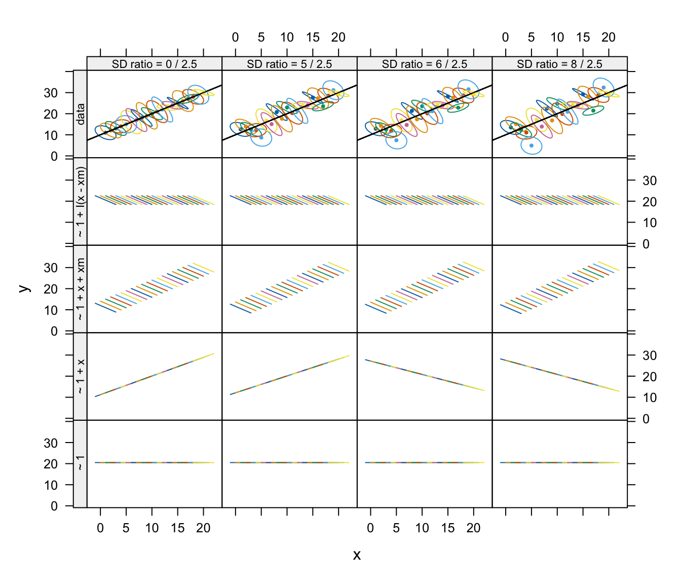

Fixed-effect predictions using each model applied to data sets with varying between- and within-patient variance ratios. The top row shows summaries of the within-patient data using estimated 50% concentration ellipses for each patient.

The BLUPs from these models are shown in the following graph:

{
  xyplot(y ~ x | SD_ratio * panel, Data,
         groups = patient, type = 'n',
         drop.unused.levels = F, 
         par.strip.text = list(cex = 0.7),
         ylab = 'fixed- and random-effect predictions (BLUPS)') +
    glayer(panel.ellipse(..., center.pch = 16, center.cex = 0.5,  
                         level = 0.5),
           panel.abline(a = 10, b = 1)) +
    xyplot(pred.BLUPs  ~ x | SD_ratio * panel, Dataf, type = 'l', 
           groups = patient,
           drop.unused.levels = F) 
}|> 
  useOuterStrips() |> print()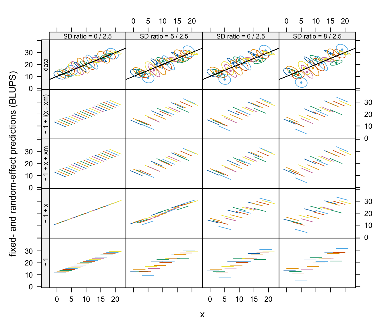

Fixed- and random-effect predictions (BLUPs) using each model applied to data sets with varying between- and within-patient variance ratios. The top row shows summaries of the within-patient data using estimated 50% concentration ellipses for each patient.

Data sets with relatively low between-patient variance result in strong shrinkage of fixed-effects predictions and also of BLUPs towards the between-patient relationship between y and x in the model with an intercept and x as fixed-effect predictors, ~ 1 + x. The inclusion of a contextual variable in the model corrects this problem.

Although the BLUPs fit the observed data more closely than predictions based on fixed effects alone, the slopes of within-patient BLUPs do not conform with the within-patient slopes for the ~ 1 + x model in the two datasets with the smallest between-patient variances.

For data with a small between-patient variance, fixed-effects predictions for the ~ 1 + x model have a slope that is close to the between-patient slope but provide better overall predictions than the fixed-effect predictions for datasets with larger between-subject variance. With data whose between-patient variance is relatively large, predictions based on the model with a common intercept and slope for all clusters, are very poor—indeed, much worse than the fixed-effects-only predictions based on the simpler random-intercept model.

We therefore anticipate (and show later in this section) that case-based cross-validation may prefer the intercept-only model, ~ 1 to the larger ~ 1 + x model when the between-cluster variance is relatively small, but that cluster-based cross-validation will prefer the latter to the former.

We will discover that case-based cross-validation prefers the ~ 1 + x model to the ~ 1 model for the ‘5 / 2.5’ dataset, but cluster-based cross-validation prefers the latter model to the former. The situation is entirely reversed with the ‘8 / 2.5’ dataset.

The third model, ~ 1 + x + xm, includes a contextual effect of x—that is, the cluster mean xm—along with x and the intercept in the fixed-effect part of the model, along with a random intercept. This model is equivalent to fitting y ~ I(x - xm) + xm + (1 | patient), which is the model that generated the data. The fit of the mixed model ~ 1 + x + xm is consequently similar to that of a fixed-effects only model with x and a categorical predictor for individual patients (i.e., y ~ factor(patient) + x, treating patients as a factor, and not shown here).

We next carry out case-based cross-validation, which, as we have explained, is based on both fixed and predicted random effects (i.e., BLUPs), and cluster-based cross-validation, which is based on fixed effects only. In order to reduce between-model random variability in comparisons of models on the same dataset, we apply cv() to the list of models created by the models() function (introduced previously), performing cross-validation with the same folds for each model.


model_lists <- lapply(fits, function(fitlist) do.call(models, fitlist))

cvs_cases <-
  lapply(1:Nv,
         function(i){
           cv(model_lists[[i]], k = 10, 
              data = split(Data, ~ SD_ratio)[[i]])
         })
#> R RNG seed set to 982470
#> R RNG seed set to 903914
#> R RNG seed set to 246168
#> R RNG seed set to 948407

cvs_clusters <-
  lapply(1:Nv,
         function(i){
           cv(model_lists[[i]],  k = 10, 
              data = split(Data, ~SD_ratio)[[i]], 
              clusterVariables = 'patient')
         })
#> R RNG seed set to 382198
#> R RNG seed set to 533366
#> R RNG seed set to 637459
#> R RNG seed set to 542289

For a given dataset, we can plot the results for a list of models using the plot method for "cvList" objects. For example

plot(cvs_clusters[[2]], main="Comparison of Fixed Effects")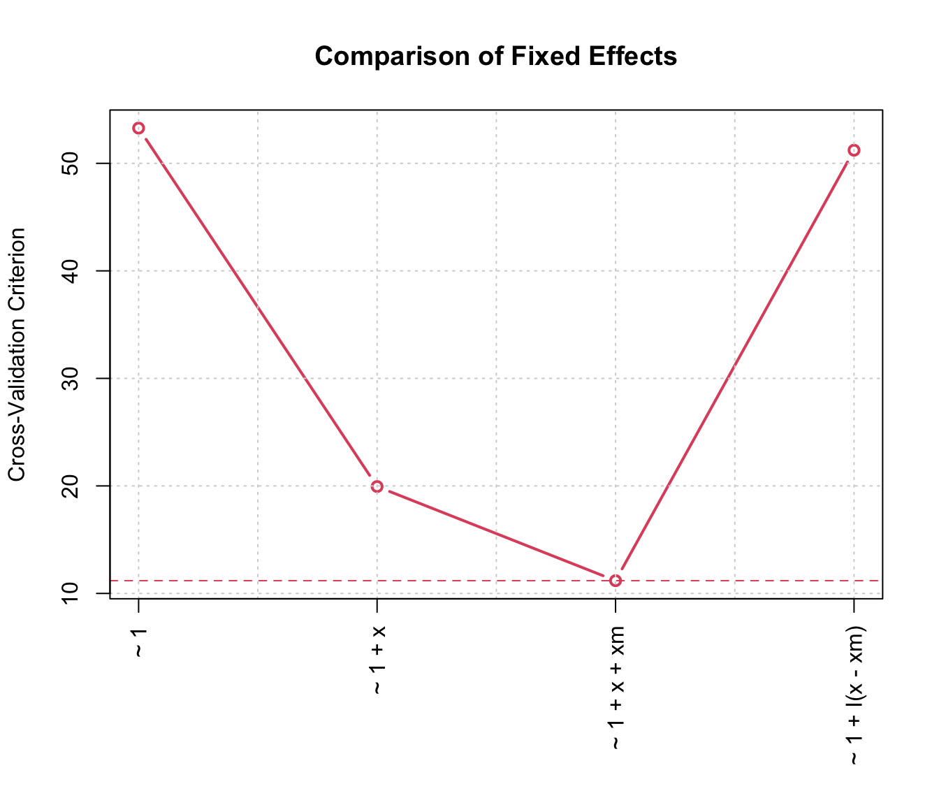

10-fold cluster-based cross-validation comparing random intercept mixed models with varying fixed effects.

We assemble the results for all datasets to show them in a common figure.

names(cvs_clusters) <- names(cvs_cases) <- SD_ratio 
dsummary <- expand.grid(SD_ratio_i = names(cvs_cases), model = names(cvs_cases[[1]]))

dsummary$cases <-
  sapply(1:nrow(dsummary), function(i){
    with(dsummary[i,], cvs_cases[[SD_ratio_i]][[model]][['CV crit']])
  })

dsummary$clusters <-
  sapply(1:nrow(dsummary), function(i){
    with(dsummary[i,], cvs_clusters[[SD_ratio_i]][[model]][['CV crit']])
  })

xyplot(cases + clusters ~ model|SD_ratio_i, dsummary,
       auto.key = list(space = 'top', reverse.rows = T, columns = 2), type = 'b',
       xlab = "Fixed Effects",
       ylab = 'CV criterion (MSE)',
       layout= c(Nv,1),
       par.settings =
         list(superpose.line=list(lty = c(2, 3), lwd = 3),
              superpose.symbol=list(pch = 15:16, cex = 1.5)),
       scales = list(y = list(log = TRUE), x = list(alternating = F, rot = 60))) |> print()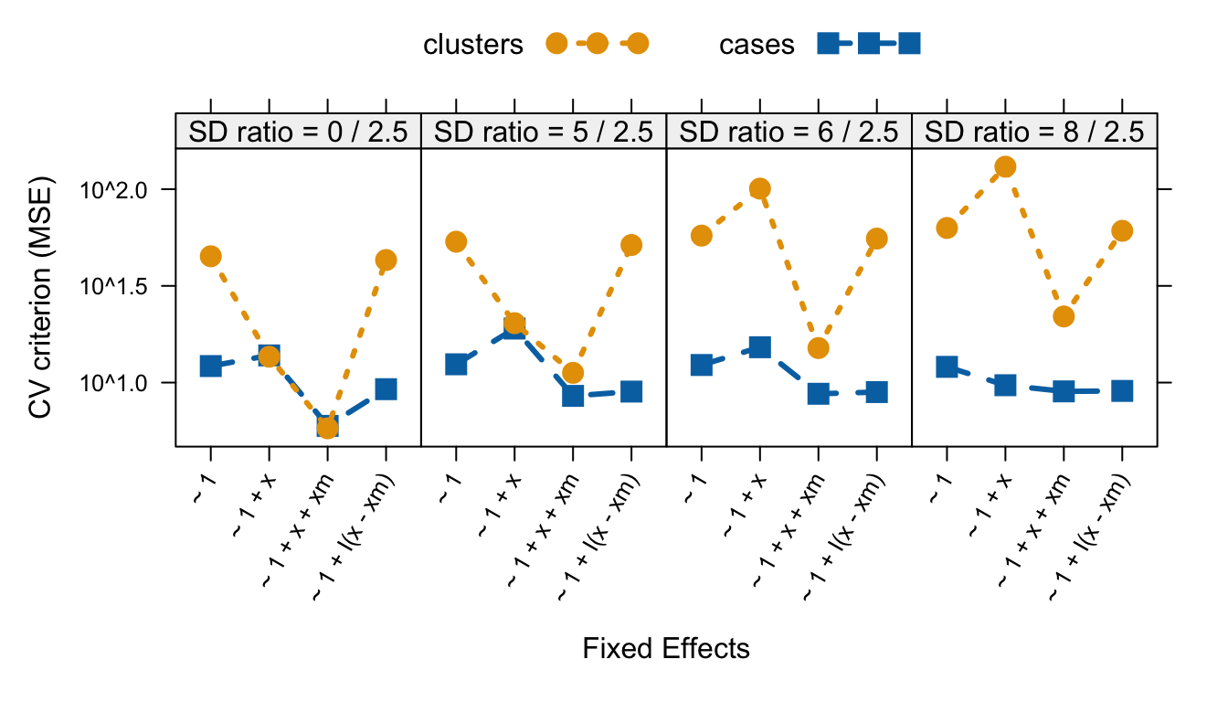

10-fold cluster- and case-based cross-validation comparing mixed models with random intercepts and various fixed effects.

In summary, when between-cluster variance is relatively large, the model ~ 1 + x, with x alone and without the contextual mean of x, is assessed as fitting very poorly by cluster-based CV, but relatively much better by case-based CV. In all our examples, the model ~ 1 + x + xm, which includes both x and its contextual mean, produces better results using both cluster-based and case-based CV. These conclusions are consistent with our observations based on graphing predictions from the various models, and they illustrate the desirability of assessing mixed-effect models at different hierarchical levels.

Example: Crossed random effects

Crossed random effects arise when the structure of the data aren’t strictly hierarchical. Nevertheless, crossed and nested random effects can be handled in much the same manner, by refitting the mixed-effects model to the data with a fold of clusters or cases removed and using the refitted model to predict the response in the removed fold.

We’ll illustrate with data on pig growth, introduced by Diggle, Liang, & Zeger (1994, Table 3.1). The data are in the Pigs data frame in the cv package:

head(Pigs, 9)
#>   id week weight
#> 1  1    1   24.0
#> 2  1    2   32.0
#> 3  1    3   39.0
#> 4  1    4   42.5
#> 5  1    5   48.0
#> 6  1    6   54.5
#> 7  1    7   61.0
#> 8  1    8   65.0
#> 9  1    9   72.0
head(xtabs( ~ id + week, data = Pigs), 3)
#>    week
#> id  1 2 3 4 5 6 7 8 9
#>   1 1 1 1 1 1 1 1 1 1
#>   2 1 1 1 1 1 1 1 1 1
#>   3 1 1 1 1 1 1 1 1 1
tail(xtabs( ~ id + week, data = Pigs), 3)
#>     week
#> id   1 2 3 4 5 6 7 8 9
#>   46 1 1 1 1 1 1 1 1 1
#>   47 1 1 1 1 1 1 1 1 1
#>   48 1 1 1 1 1 1 1 1 1

Each of 48 pigs is observed weekly over a period of 9 weeks, with the weight of the pig recorded in kg. The data are in “long” format, as is appropriate for use with the lmer() function in the lme4 package. The data are very regular, with no missing cases.

The following graph, showing the growth trajectories of the pigs, is similar to Figure 3.1 in Diggle et al. (1994); we add an overall least-squares line and a loess smooth, which are nearly indistinguishable:

plot(weight ~ week, data = Pigs, type = "n")
for (i in unique(Pigs$id)) {
  with(Pigs, lines(
    x = 1:9,
    y = Pigs[id == i, "weight"],
    col = "gray"
  ))
}
abline(lm(weight ~ week, data = Pigs),
       col = "blue",
       lwd = 2)
lines(
  with(Pigs, loess.smooth(week, weight, span = 0.5)),
  col = "magenta",
  lty = 2,
  lwd = 2
)

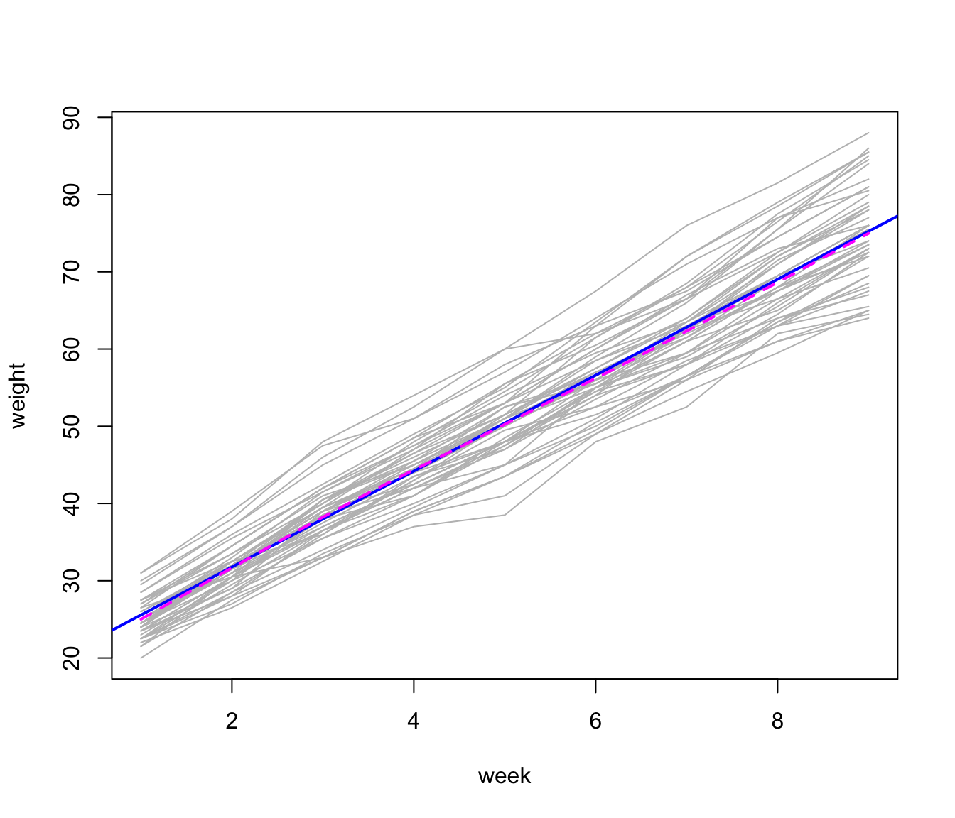
Growth trajectories for 48 pigs, with overall least-squares line (sold blue) and loess line (broken magenta).

The individual “growth curves” and the overall trend are generally linear, with some tendency for variability of pig weight to increase over weeks (a feature of the data that we ignore in the mixed model that we fit to the data below).

The Stata mixed-effects models manual proposes a model with crossed random effects for the Pigs data (StataCorp LLC, 2023, p. 37):

[S]uppose that we wish to fit $\mathrm{weight}_{ij} = \beta_0 + \beta_1 \mathrm{week}_{ij} + u_i + v_j + \varepsilon_{ij}$ for the $i = 1, \ldots, 9$ weeks and $j = 1, \dots, 48$ pigs and $u_i \sim N(0, \sigma^2_u); v_j \sim N(0, \sigma^2_v ); \varepsilon_{ij} \sim N(0, \sigma^2_\varepsilon)$ all independently. That is, we assume an overall population-average growth curve $\beta_0 + \beta_1 \mathrm{week}$ and a random pig-specific shift. In other words, the effect due to week, $u_i$ , is systematic to that week and common to all pigs. The rationale behind [this model] could be that, assuming that the pigs were measured contemporaneously, we might be concerned that week-specific random factors such as weather and feeding patterns had significant systematic effects on all pigs.

Although we might prefer an alternative model,⁶ we think that this is a reasonable specification.

The Stata manual fits the mixed model by maximum likelihood (rather than REML), and we duplicate the results reported there using lmer():

m.p <- lmer(
  weight ~ week + (1 | id) + (1 | week),
  data = Pigs,
  REML = FALSE, # i.e., ML
  control = lmerControl(optimizer = "bobyqa")
)
summary(m.p)
#> Linear mixed model fit by maximum likelihood  ['lmerMod']
#> Formula: weight ~ week + (1 | id) + (1 | week)
#>    Data: Pigs
#> Control: lmerControl(optimizer = "bobyqa")
#> 
#>      AIC      BIC   logLik deviance df.resid 
#>   2037.6   2058.0  -1013.8   2027.6      427 
#> 
#> Scaled residuals: 
#>    Min     1Q Median     3Q    Max 
#> -3.775 -0.542  0.005  0.476  3.982 
#> 
#> Random effects:
#>  Groups   Name        Variance Std.Dev.
#>  id       (Intercept) 14.836   3.852   
#>  week     (Intercept)  0.085   0.292   
#>  Residual              4.297   2.073   
#> Number of obs: 432, groups:  id, 48; week, 9
#> 
#> Fixed effects:
#>             Estimate Std. Error t value
#> (Intercept)  19.3556     0.6334    30.6
#> week          6.2099     0.0539   115.1
#> 
#> Correlation of Fixed Effects:
#>      (Intr)
#> week -0.426

We opt for the non-default "bobyqa" optimizer because it provides more numerically stable results for subsequent cross-validation in this example.

We can then cross-validate the model by omitting folds composed of pigs, folds composed of weeks, or folds composed of pig-weeks (which in the Pigs data set correspond to individual cases, using only the fixed effects):

cv(m.p, clusterVariables = "id")
#> n-Fold Cross Validation based on 48 {id} clusters
#> criterion: mse
#> cross-validation criterion = 19.973
#> bias-adjusted cross-validation criterion = 19.965
#> 95% CI for bias-adjusted CV criterion = (17.125, 22.805)
#> full-sample criterion = 19.201

cv(m.p, clusterVariables = "week")
#> boundary (singular) fit: see help('isSingular')
#> n-Fold Cross Validation based on 9 {week} clusters
#> criterion: mse
#> cross-validation criterion = 19.312
#> bias-adjusted cross-validation criterion = 19.305
#> 95% CI for bias-adjusted CV criterion = (16.566, 22.044)
#> full-sample criterion = 19.201

cv(
  m.p,
  clusterVariables = c("id", "week"),
  k = 10,
  seed = 8469
)
#> R RNG seed set to 8469
#> 10-Fold Cross Validation based on 432 {id, week} clusters
#> criterion: mse
#> cross-validation criterion = 19.235
#> bias-adjusted cross-validation criterion = 19.233
#> 95% CI for bias-adjusted CV criterion = (16.493, 21.973)
#> full-sample criterion = 19.201

We can also cross-validate the individual cases taking account of the random effects (employing the same 10 folds):

cv(m.p, k = 10, seed = 8469)
#> R RNG seed set to 8469
#> 10-Fold Cross Validation
#> criterion: mse
#> cross-validation criterion = 5.1583
#> bias-adjusted cross-validation criterion = 5.0729
#> 95% CI for bias-adjusted CV criterion = (4.123, 6.0229)
#> full-sample criterion = 3.796

Because these predictions are based on BLUPs, they are more accurate than the predictions based only on fixed effects.⁷ As well, the difference between the MSE computed for the model fit to the full data and the CV estimates of the MSE is greater here than for cluster-based predictions.

References

Bates, D., Mächler, M., Bolker, B., & Walker, S. (2015). Fitting linear mixed-effects models using lme4. Journal of Statistical Software, 67(1), 1–48.

Brooks, M. E., Kristensen, K., van Benthem, K. J., Magnusson, A., Berg, C. W., Nielsen, A., … Bolker, B. M. (2017). glmmTMB balances speed and flexibility among packages for zero-inflated generalized linear mixed modeling. The R Journal, 9(2), 378–400. http://doi.org/10.32614/RJ-2017-066

Diggle, P. J., Liang, K.-Y., & Zeger, S. L. (1994). Analysis of longitudinal data. Oxford: Oxford University Press.

Fox, J., & Weisberg, S. (2019). An R companion to applied regression (Third edition). Thousand Oaks CA: Sage.

Pinheiro, J. C., & Bates, D. M. (2000). Mixed-effects models in S and S-PLUS. New York: Springer.

Raudenbush, S. W., & Bryk, A. S. (2002). Hierarchical linear models: Applications and data analysis methods (Second edition). Thousand Oaks CA: Sage.

Sarkar, D. (2008). Lattice: Multivariate data visualization with R. New York: Springer. Retrieved from http://lmdvr.r-forge.r-project.org

Sarkar, D., & Andrews, F. (2022). latticeExtra: Extra graphical utilities based on lattice. Retrieved from https://CRAN.R-project.org/package=latticeExtra

StataCorp LLC. (2023). Stata multilevel mixed-effects reference manual, release 18. College Station TX: Stata Press. Retrieved from https://www.stata.com/manuals/me.pdf

Vehtari, A. (2023). Cross-validation FAQ. Retrieved October 15, 2023, from https://users.aalto.fi/~ave/CV-FAQ.html

Wickham, H., François, R., Henry, L., Müller, K., & Vaughan, D. (2023). Dplyr: A grammar of data manipulation. Retrieved from https://CRAN.R-project.org/package=dplyr

John Fox and Georges Monette

2024-07-26

Example: The High-School and Beyond data

Example: Contrasting cluster-based and case-based CV

Example: Crossed random effects

References