Cross-validating model selection

John Fox and Georges Monette

2024-10-16

As Hastie, Tibshirani, & Friedman (2009, sec. 7.10.2: “The Wrong and Right Way to Do Cross-validation”) explain, if the whole data are used to select or fine-tune a statistical model, subsequent cross-validation of the model is intrinsically misleading, because the model is selected to fit the whole data, including the part of the data that remains when each fold is removed.

A preliminary example

The following example is similar in spirit to one employed by Hastie et al. (2009). Suppose that we randomly generate $n = 1000$ independent observations for a response variable variable $y \sim N(\mu = 10, \sigma^2 = 0)$, and independently sample $1000$ observations for $p = 100$ “predictors,” $x_1, \ldots, x_{100}$, each from $x_j \sim N(0, 1)$. The response has nothing to do with the predictors and so the population linear-regression model $y_i = \alpha + \beta_1 x_{i1} + \cdots + \beta_{100} x_{i,100} + \varepsilon_i$ has $\alpha = 10$ and all $\beta_j = 0$.

set.seed(24361) # for reproducibility
D <- data.frame(y = rnorm(1000, mean = 10),
                X = matrix(rnorm(1000 * 100), 1000, 100))
head(D[, 1:6])
#>         y      X.1      X.2      X.3       X.4       X.5
#> 1 10.0316 -1.23886 -0.26487 -0.03539 -2.576973  0.811048
#> 2  9.6650  0.12287 -0.17744  0.37290 -0.935138  0.628673
#> 3 10.0232 -0.95052 -0.73487 -1.05978  0.882944  0.023918
#> 4  8.9910  1.13571  0.32411  0.11037  1.376303 -0.422114
#> 5  9.0712  1.49474  1.87538  0.10575  0.292140 -0.184568
#> 6 11.3493 -0.18453 -0.78037 -1.23804 -0.010949  0.691034

Least-squares provides accurate estimates of the regression constant $\alpha = 10$ and the error variance $\sigma^2 = 1$ for the “null model” including only the regression constant; moreover, the omnibus $F$-test of the correct null hypothesis that all of the $\beta$s are 0 for the “full model” with all 100 $x$s is associated with a large $p$-value:

m.full <- lm(y ~ ., data = D)
m.null <- lm(y ~ 1, data = D)
anova(m.null, m.full)
#> Analysis of Variance Table
#> 
#> Model 1: y ~ 1
#> Model 2: y ~ X.1 + X.2 + X.3 + X.4 + X.5 + X.6 + X.7 + X.8 + X.9 + X.10 + 
#>     X.11 + X.12 + X.13 + X.14 + X.15 + X.16 + X.17 + X.18 + X.19 + 
#>     X.20 + X.21 + X.22 + X.23 + X.24 + X.25 + X.26 + X.27 + X.28 + 
#>     X.29 + X.30 + X.31 + X.32 + X.33 + X.34 + X.35 + X.36 + X.37 + 
#>     X.38 + X.39 + X.40 + X.41 + X.42 + X.43 + X.44 + X.45 + X.46 + 
#>     X.47 + X.48 + X.49 + X.50 + X.51 + X.52 + X.53 + X.54 + X.55 + 
#>     X.56 + X.57 + X.58 + X.59 + X.60 + X.61 + X.62 + X.63 + X.64 + 
#>     X.65 + X.66 + X.67 + X.68 + X.69 + X.70 + X.71 + X.72 + X.73 + 
#>     X.74 + X.75 + X.76 + X.77 + X.78 + X.79 + X.80 + X.81 + X.82 + 
#>     X.83 + X.84 + X.85 + X.86 + X.87 + X.88 + X.89 + X.90 + X.91 + 
#>     X.92 + X.93 + X.94 + X.95 + X.96 + X.97 + X.98 + X.99 + X.100
#>   Res.Df RSS  Df Sum of Sq    F Pr(>F)
#> 1    999 974                          
#> 2    899 888 100      85.2 0.86   0.82

summary(m.null)
#> 
#> Call:
#> lm(formula = y ~ 1, data = D)
#> 
#> Residuals:
#>    Min     1Q Median     3Q    Max 
#> -3.458 -0.681  0.019  0.636  2.935 
#> 
#> Coefficients:
#>             Estimate Std. Error t value Pr(>|t|)    
#> (Intercept)   9.9370     0.0312     318   <2e-16 ***
#> ---
#> Signif. codes:  0 '***' 0.001 '**' 0.01 '*' 0.05 '.' 0.1 ' ' 1
#> 
#> Residual standard error: 0.987 on 999 degrees of freedom

Next, using the stepAIC() function in the MASS package (Venables & Ripley, 2002), let us perform a forward stepwise regression to select a “best” model, starting with the null model, and using AIC as the model-selection criterion (see the help page for stepAIC() for details):¹

library("MASS")  # for stepAIC()
m.select <- stepAIC(
  m.null,
  direction = "forward",
  trace = FALSE,
  scope = list(lower =  ~ 1, upper = formula(m.full))
)
summary(m.select)
#> 
#> Call:
#> lm(formula = y ~ X.99 + X.90 + X.87 + X.40 + X.65 + X.91 + X.53 + 
#>     X.45 + X.31 + X.56 + X.61 + X.60 + X.46 + X.35 + X.92, data = D)
#> 
#> Residuals:
#>    Min     1Q Median     3Q    Max 
#> -3.262 -0.645  0.024  0.641  3.118 
#> 
#> Coefficients:
#>             Estimate Std. Error t value Pr(>|t|)    
#> (Intercept)   9.9372     0.0310  320.80   <2e-16 ***
#> X.99         -0.0910     0.0308   -2.95   0.0032 ** 
#> X.90         -0.0820     0.0314   -2.62   0.0090 ** 
#> X.87         -0.0694     0.0311   -2.24   0.0256 *  
#> X.40         -0.0476     0.0308   -1.55   0.1221    
#> X.65         -0.0552     0.0315   -1.76   0.0795 .  
#> X.91          0.0524     0.0308    1.70   0.0894 .  
#> X.53         -0.0492     0.0305   -1.61   0.1067    
#> X.45          0.0554     0.0318    1.74   0.0818 .  
#> X.31          0.0452     0.0311    1.46   0.1457    
#> X.56          0.0543     0.0327    1.66   0.0972 .  
#> X.61         -0.0508     0.0317   -1.60   0.1091    
#> X.60         -0.0513     0.0319   -1.61   0.1083    
#> X.46          0.0516     0.0327    1.58   0.1153    
#> X.35          0.0470     0.0315    1.49   0.1358    
#> X.92          0.0443     0.0310    1.43   0.1533    
#> ---
#> Signif. codes:  0 '***' 0.001 '**' 0.01 '*' 0.05 '.' 0.1 ' ' 1
#> 
#> Residual standard error: 0.973 on 984 degrees of freedom
#> Multiple R-squared:  0.0442, Adjusted R-squared:  0.0296 
#> F-statistic: 3.03 on 15 and 984 DF,  p-value: 8.34e-05

library("cv")
#> Loading required package: doParallel
#> Loading required package: foreach
#> Loading required package: iterators
#> Loading required package: parallel
mse(D$y, fitted(m.select))
#> [1] 0.93063
#> attr(,"casewise loss")
#> [1] "(y - yhat)^2"

The resulting model has 15 predictors, a very modest $R^2 = .044$, but a small $p$-value for its omnibus $F$-test (which, of course, is entirely spurious because the same data were used to select and test the model). The MSE for the selected model is smaller than the true error variance $\sigma^2 = 1$, as is the estimated error variance for the selected model, $\widehat{\sigma}^2 = 0.973^2 = 0.947$.

If we cross-validate the selected model, we also obtain an optimistic estimate of its predictive power (although the confidence interval for the bias-adjusted MSE includes 1):

library("cv")

summary(cv(m.select, seed = 2529))
#> R RNG seed set to 2529
#> 10-Fold Cross Validation
#> method: Woodbury
#> criterion: mse
#> cross-validation criterion = 0.95937
#> bias-adjusted cross-validation criterion = 0.95785
#> 95% CI for bias-adjusted CV criterion = (0.87661, 1.0391)
#> full-sample criterion = 0.93063

The "function" method of cv() allows us to cross-validate the whole model-selection procedure, where first argument to cv() is a model-selection function capable of refitting the model with a fold omitted and returning a CV criterion. The selectStepAIC() function, in the cv package and based on stepAIC(), is suitable for use with cv():

cv.select <- cv(
  selectStepAIC,
  data = D,
  seed = 3791,
  working.model = m.null,
  direction = "forward",
  scope = list(lower =  ~ 1, upper = formula(m.full))
)
#> R RNG seed set to 3791
summary(cv.select)
#> 10-Fold Cross Validation
#> criterion: mse
#> cross-validation criterion = 1.0687
#> bias-adjusted cross-validation criterion = 1.0612
#> 95% CI for bias-adjusted CV criterion = (0.97172, 1.1506)
#> full-sample criterion = 0.93063

The other arguments to cv() are:

• data, the data set to which the model is fit;
• seed, an optional seed for R’s pseudo-random-number generator; as for cv(), if the seed isn’t supplied by the user, a seed is randomly selected and saved;
• additional arguments required by the model-selection function, here the starting working.model argument, the direction of model selection, and the scope of models considered (from the model with only a regression constant to the model with all 100 predictors).

By default, cv() performs 10-fold CV, and produces an estimate of MSE for the model-selection procedure even larger than the true error variance, $\sigma^2 = 1$.

Also by default, when the number of folds is 10 or fewer, cv() saves details data about the folds. In this example, the compareFolds() function reveals that the variables retained by the model-selection process in the several folds are quite different:

compareFolds(cv.select)
#> CV criterion by folds:
#>  fold.1  fold.2  fold.3  fold.4  fold.5  fold.6  fold.7  fold.8  fold.9 fold.10 
#> 1.26782 1.12837 1.04682 1.31007 1.06899 0.87916 0.88380 0.95026 1.21070 0.94130 
#> 
#> Coefficients by folds:
#>         (Intercept)    X.87    X.90    X.99    X.91    X.54    X.53    X.56
#> Fold 1       9.9187 -0.0615 -0.0994 -0.0942  0.0512  0.0516                
#> Fold 2       9.9451 -0.0745 -0.0899 -0.0614          0.0587          0.0673
#> Fold 3       9.9423 -0.0783 -0.0718 -0.0987  0.0601                  0.0512
#> Fold 4       9.9410 -0.0860 -0.0831 -0.0867  0.0570         -0.0508        
#> Fold 5       9.9421 -0.0659 -0.0849 -0.1004  0.0701  0.0511 -0.0487  0.0537
#> Fold 6       9.9633 -0.0733 -0.0874 -0.0960  0.0555  0.0629 -0.0478        
#> Fold 7       9.9279 -0.0618 -0.0960 -0.0838  0.0533         -0.0464        
#> Fold 8       9.9453 -0.0610 -0.0811 -0.0818          0.0497 -0.0612  0.0560
#> Fold 9       9.9173 -0.0663 -0.0894 -0.1100  0.0504  0.0524          0.0747
#> Fold 10      9.9449 -0.0745 -0.0906 -0.0891  0.0535  0.0482 -0.0583  0.0642
#>            X.40    X.45    X.65    X.68    X.92    X.15    X.26    X.46    X.60
#> Fold 1                  -0.0590                 -0.0456  0.0658  0.0608        
#> Fold 2                                   0.0607          0.0487                
#> Fold 3  -0.0496         -0.0664          0.0494                                
#> Fold 4  -0.0597  0.0579 -0.0531          0.0519 -0.0566                 -0.0519
#> Fold 5                           0.0587                          0.0527 -0.0603
#> Fold 6  -0.0596  0.0552          0.0474                                        
#> Fold 7           0.0572          0.0595                                        
#> Fold 8           0.0547 -0.0617  0.0453  0.0493 -0.0613  0.0591  0.0703 -0.0588
#> Fold 9  -0.0552  0.0573 -0.0635  0.0492         -0.0513  0.0484         -0.0507
#> Fold 10 -0.0558                          0.0529                  0.0710        
#>            X.61     X.8    X.28    X.29    X.31    X.35    X.70    X.89    X.17
#> Fold 1  -0.0490          0.0616 -0.0537                  0.0638                
#> Fold 2           0.0671                  0.0568                  0.0523        
#> Fold 3  -0.0631          0.0616                                                
#> Fold 4           0.0659         -0.0549          0.0527                  0.0527
#> Fold 5           0.0425                  0.0672  0.0613          0.0493        
#> Fold 6           0.0559         -0.0629  0.0498          0.0487                
#> Fold 7                                                           0.0611  0.0472
#> Fold 8  -0.0719                                          0.0586                
#> Fold 9                   0.0525                                                
#> Fold 10 -0.0580                                  0.0603                        
#>            X.25     X.4    X.64    X.81    X.97    X.11     X.2    X.33    X.47
#> Fold 1                                   0.0604          0.0575                
#> Fold 2   0.0478          0.0532  0.0518                                        
#> Fold 3                           0.0574                          0.0473        
#> Fold 4                   0.0628                                                
#> Fold 5   0.0518                                                                
#> Fold 6                                           0.0521                        
#> Fold 7           0.0550                                                        
#> Fold 8                                                                         
#> Fold 9                                   0.0556                          0.0447
#> Fold 10          0.0516                                                        
#>             X.6    X.72    X.73    X.77    X.79 X.88
#> Fold 1   0.0476                                     
#> Fold 2                   0.0514                     
#> Fold 3                                              
#> Fold 4                                  -0.0473     
#> Fold 5           0.0586                         0.07
#> Fold 6                          -0.0489             
#> Fold 7                                              
#> Fold 8                                              
#> Fold 9                                              
#> Fold 10

Polynomial regression for the Auto data revisited: meta cross-validation

In the introductory vignette on cross-validating regression models, following James, Witten, Hastie, & Tibshirani (2021, secs. 5.1, 5.3), we fit polynomial regressions up to degree 10 to the relationship of mpg to horsepower for the Auto data, saving the results in m.1 through m.10. We then used cv() to compare the cross-validated MSE for the 10 models, discovering that the 7th degree polynomial had the smallest MSE (by a small margin); repeating the relevant graph:

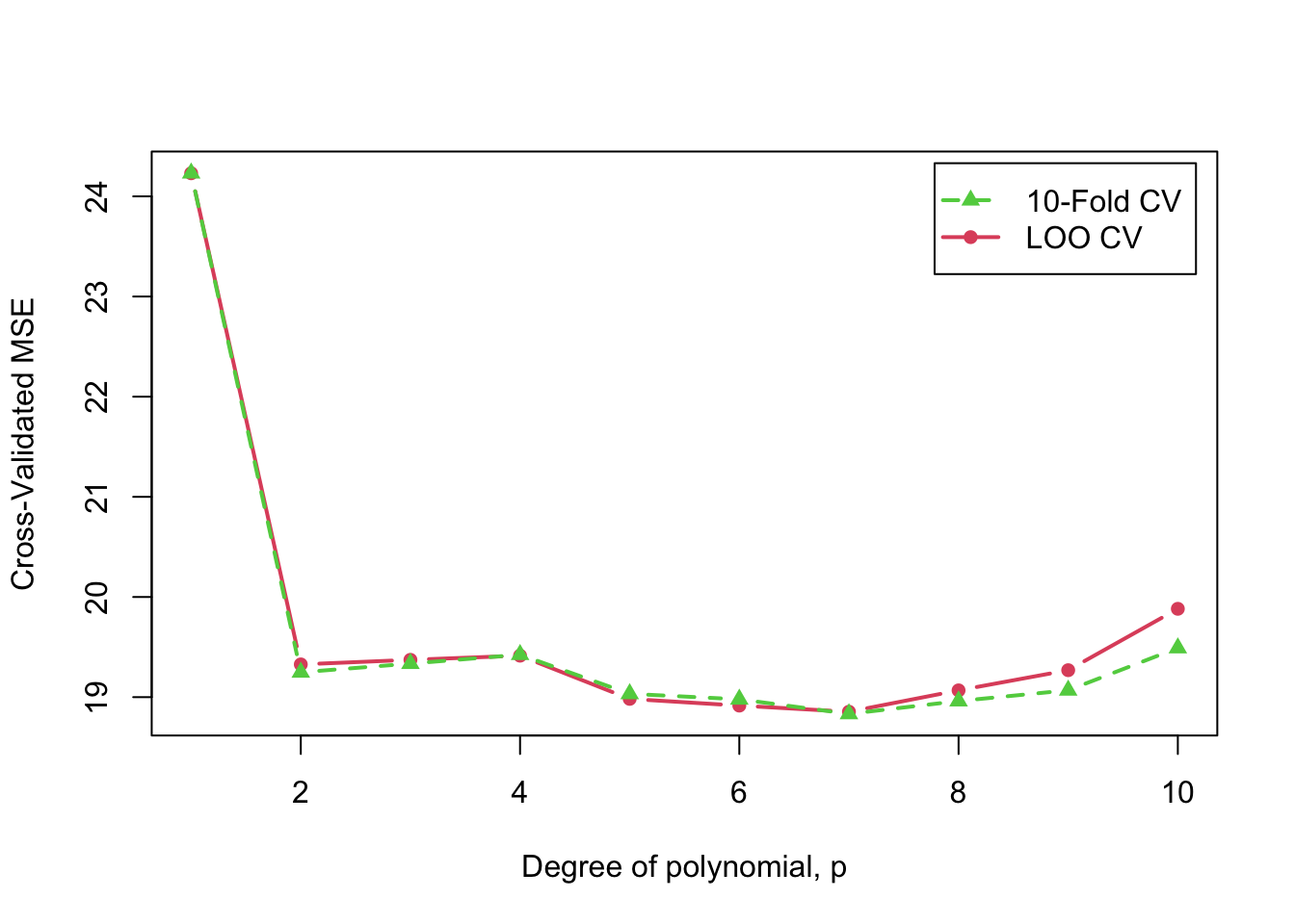
Cross-validated 10-fold and LOO MSE as a function of polynomial degree, $p$ (repeated)

If we then select the 7th degree polynomial model, intending to use it for prediction, the CV estimate of the MSE for this model will be optimistic. One solution is to cross-validate the process of using CV to select the “best” model—that is, to apply CV to CV recursively, a process that we term “meta cross-validation.” The function selectModelList(), which is suitable for use with cv(), implements this idea.

Applying selectModelList() to the Auto polynomial-regression models, and using 10-fold CV, we obtain:

metaCV.auto <- cv(
  selectModelList,
  Auto,
  working.model = models(m.1, m.2, m.3, m.4, m.5,
                         m.6, m.7, m.8, m.9, m.10),
  save.model = TRUE,
  seed = 2120
)
#> R RNG seed set to 2120
summary(metaCV.auto)
#> 10-Fold Cross Validation
#> criterion: mse
#> cross-validation criterion = 19.105
#> bias-adjusted cross-validation criterion = 19.68
#> full-sample criterion = 18.746
(m.sel <- cvInfo(metaCV.auto, "selected model"))
#> 
#> Call:
#> lm(formula = mpg ~ poly(horsepower, 7), data = Auto)
#> 
#> Coefficients:
#>          (Intercept)  poly(horsepower, 7)1  poly(horsepower, 7)2  
#>                23.45               -120.14                 44.09  
#> poly(horsepower, 7)3  poly(horsepower, 7)4  poly(horsepower, 7)5  
#>                -3.95                 -5.19                 13.27  
#> poly(horsepower, 7)6  poly(horsepower, 7)7  
#>                -8.55                  7.98
cv(m.sel, seed = 2120) # same seed for same folds
#> R RNG seed set to 2120
#> cross-validation criterion (mse) = 18.898

As expected, meta CV produces a larger estimate of MSE for the selected 7th degree polynomial model than CV applied directly to this model.

We can equivalently call cv() with the list of models as the first argument and set meta=TRUE:

metaCV.auto.alt <- cv(
  models(m.1, m.2, m.3, m.4, m.5,
         m.6, m.7, m.8, m.9, m.10),
  data = Auto,
  seed = 2120,
  meta = TRUE,
  save.model = TRUE
)
#> R RNG seed set to 2120
all.equal(metaCV.auto, metaCV.auto.alt)
#> [1] "Component \"criterion\": 1 string mismatch"

Mroz’s logistic regression revisited

Next, let’s apply model selection to Mroz’s logistic regression for married women’s labor-force participation, also discussed in the introductory vignette on cross-validating regression models. First, recall the logistic regression model that we fit to the Mroz data:

data("Mroz", package = "carData")
m.mroz <- glm(lfp ~ ., data = Mroz, family = binomial)
summary(m.mroz)
#> 
#> Call:
#> glm(formula = lfp ~ ., family = binomial, data = Mroz)
#> 
#> Coefficients:
#>             Estimate Std. Error z value Pr(>|z|)    
#> (Intercept)  3.18214    0.64438    4.94  7.9e-07 ***
#> k5          -1.46291    0.19700   -7.43  1.1e-13 ***
#> k618        -0.06457    0.06800   -0.95  0.34234    
#> age         -0.06287    0.01278   -4.92  8.7e-07 ***
#> wcyes        0.80727    0.22998    3.51  0.00045 ***
#> hcyes        0.11173    0.20604    0.54  0.58762    
#> lwg          0.60469    0.15082    4.01  6.1e-05 ***
#> inc         -0.03445    0.00821   -4.20  2.7e-05 ***
#> ---
#> Signif. codes:  0 '***' 0.001 '**' 0.01 '*' 0.05 '.' 0.1 ' ' 1
#> 
#> (Dispersion parameter for binomial family taken to be 1)
#> 
#>     Null deviance: 1029.75  on 752  degrees of freedom
#> Residual deviance:  905.27  on 745  degrees of freedom
#> AIC: 921.3
#> 
#> Number of Fisher Scoring iterations: 4

Applying stepwise model selection Mroz’s logistic regression, using BIC as the model-selection criterion (via the argument k=log(nrow(Mroz)) to stepAIC()) selects 5 of the 7 original predictors:

m.mroz.sel <- stepAIC(m.mroz, k = log(nrow(Mroz)),
                      trace = FALSE)
summary(m.mroz.sel)
#> 
#> Call:
#> glm(formula = lfp ~ k5 + age + wc + lwg + inc, family = binomial, 
#>     data = Mroz)
#> 
#> Coefficients:
#>             Estimate Std. Error z value Pr(>|z|)    
#> (Intercept)   2.9019     0.5429    5.35  9.0e-08 ***
#> k5           -1.4318     0.1932   -7.41  1.3e-13 ***
#> age          -0.0585     0.0114   -5.13  2.9e-07 ***
#> wcyes         0.8724     0.2064    4.23  2.4e-05 ***
#> lwg           0.6157     0.1501    4.10  4.1e-05 ***
#> inc          -0.0337     0.0078   -4.32  1.6e-05 ***
#> ---
#> Signif. codes:  0 '***' 0.001 '**' 0.01 '*' 0.05 '.' 0.1 ' ' 1
#> 
#> (Dispersion parameter for binomial family taken to be 1)
#> 
#>     Null deviance: 1029.75  on 752  degrees of freedom
#> Residual deviance:  906.46  on 747  degrees of freedom
#> AIC: 918.5
#> 
#> Number of Fisher Scoring iterations: 3
BayesRule(Mroz$lfp == "yes",
          predict(m.mroz.sel, type = "response"))
#> [1] 0.31873
#> attr(,"casewise loss")
#> [1] "y != round(yhat)"

Bayes rule applied to the selected model misclassifies 32% of the cases in the Mroz data.

Cross-validating the selected model produces a similar, slightly larger, estimate of misclassification, about 33%:

summary(cv(m.mroz.sel, criterion = BayesRule, seed = 345266))
#> R RNG seed set to 345266
#> 10-Fold Cross Validation
#> method: exact
#> criterion: BayesRule
#> cross-validation criterion = 0.33068
#> bias-adjusted cross-validation criterion = 0.33332
#> 95% CI for bias-adjusted CV criterion = (0.2997, 0.36695)
#> full-sample criterion = 0.31873

Is this estimate of predictive performance optimistic?

We proceed to apply the model-selection procedure by cross-validation, producing more or less the same result:

m.mroz.sel.cv <- cv(
  selectStepAIC,
  Mroz,
  seed = 6681,
  criterion = BayesRule,
  working.model = m.mroz,
  AIC = FALSE
)
#> R RNG seed set to 6681
summary(m.mroz.sel.cv)
#> 10-Fold Cross Validation
#> criterion: BayesRule
#> cross-validation criterion = 0.33068
#> bias-adjusted cross-validation criterion = 0.33452
#> 95% CI for bias-adjusted CV criterion = (0.3009, 0.36815)
#> full-sample criterion = 0.31873

Setting AIC=FALSE in the call to cv() uses the BIC rather than the AIC as the model-selection criterion. As it turns out, exactly the same predictors are selected when each of the 10 folds are omitted, and the several coefficient estimates are very similar, as we show using compareFolds():

compareFolds(m.mroz.sel.cv)
#> CV criterion by folds:
#>  fold.1  fold.2  fold.3  fold.4  fold.5  fold.6  fold.7  fold.8  fold.9 fold.10 
#> 0.27632 0.40789 0.34211 0.36000 0.28000 0.37333 0.32000 0.29333 0.33333 0.32000 
#> 
#> Coefficients by folds:
#>         (Intercept)     age     inc      k5     lwg wcyes
#> Fold 1       2.5014 -0.0454 -0.0388 -1.3613  0.5653  0.85
#> Fold 2       3.0789 -0.0659 -0.0306 -1.5335  0.6923  0.79
#> Fold 3       3.0141 -0.0595 -0.0305 -1.3994  0.5428  0.86
#> Fold 4       2.7251 -0.0543 -0.0354 -1.4474  0.6298  1.09
#> Fold 5       2.7617 -0.0566 -0.0320 -1.4752  0.6324  0.74
#> Fold 6       3.0234 -0.0621 -0.0348 -1.4537  0.6618  0.94
#> Fold 7       2.9615 -0.0600 -0.0351 -1.4127  0.5835  0.97
#> Fold 8       2.9598 -0.0603 -0.0329 -1.3865  0.6210  0.69
#> Fold 9       3.2481 -0.0650 -0.0381 -1.4138  0.6093  0.94
#> Fold 10      2.7724 -0.0569 -0.0295 -1.4503  0.6347  0.85

In this example, therefore, we appear to obtain a realistic estimate of model performance directly from the selected model, because there is little added uncertainty induced by model selection.

Cross-validating choice of transformations in regression

The cv package also provides a cv() procedure, selectTrans(), for choosing transformations of the predictors and the response in regression.

Some background: As Weisberg (2014, sec. 8.2) explains, there are technical advantages to having (numeric) predictors in linear regression analysis that are themselves linearly related. If the predictors aren’t linearly related, then the relationships between them can often be straightened by power transformations. Transformations can be selected after graphical examination of the data, or by analytic methods. Once the relationships between the predictors are linearized, it can be advantageous similarly to transform the response variable towards normality.

Selecting transformations analytically raises the possibility of automating the process, as would be required for cross-validation. One could, in principle, apply graphical methods to select transformations for each fold, but because a data analyst couldn’t forget the choices made for previous folds, the process wouldn’t really be applied independently to the folds.

To illustrate, we adapt an example appearing in several places in Fox & Weisberg (2019) (for example in Chapter 3 on transforming data), using data on the prestige and other characteristics of 102 Canadian occupations circa 1970. The data are in the Prestige data frame in the carData package:

data("Prestige", package = "carData")
head(Prestige)
#>                     education income women prestige census type
#> gov.administrators      13.11  12351 11.16     68.8   1113 prof
#> general.managers        12.26  25879  4.02     69.1   1130 prof
#> accountants             12.77   9271 15.70     63.4   1171 prof
#> purchasing.officers     11.42   8865  9.11     56.8   1175 prof
#> chemists                14.62   8403 11.68     73.5   2111 prof
#> physicists              15.64  11030  5.13     77.6   2113 prof
summary(Prestige)
#>    education         income          women          prestige        census    
#>  Min.   : 6.38   Min.   :  611   Min.   : 0.00   Min.   :14.8   Min.   :1113  
#>  1st Qu.: 8.45   1st Qu.: 4106   1st Qu.: 3.59   1st Qu.:35.2   1st Qu.:3120  
#>  Median :10.54   Median : 5930   Median :13.60   Median :43.6   Median :5135  
#>  Mean   :10.74   Mean   : 6798   Mean   :28.98   Mean   :46.8   Mean   :5402  
#>  3rd Qu.:12.65   3rd Qu.: 8187   3rd Qu.:52.20   3rd Qu.:59.3   3rd Qu.:8312  
#>  Max.   :15.97   Max.   :25879   Max.   :97.51   Max.   :87.2   Max.   :9517  
#>    type   
#>  bc  :44  
#>  prof:31  
#>  wc  :23  
#>  NA's: 4  
#>           
#> 

The variables in the Prestige data set are:

• education: average years of education for incumbents in the occupation, from the 1971 Canadian Census.
• income: average dollars of annual income for the occupation, from the Census.
• women: percentage of occupational incumbents who were women, also from the Census.
• prestige: the average prestige rating of the occupation on a 0–100 “thermometer” scale, in a Canadian social survey conducted around the same time.
• type, type of occupation, and census, the Census occupational code, which are not used in our example.

The object of a regression analysis for the Prestige data (and their original purpose) is to predict occupational prestige from the other variables in the data set.

A scatterplot matrix (using the scatterplotMatrix() function in the car package) of the numeric variables in the data reveals that the distributions of income and women are positively skewed, and that some of the relationships among the three predictors, and between the predictors and the response (i.e., prestige), are nonlinear:

library("car")
#> Loading required package: carData
scatterplotMatrix(
  ~ prestige + income + education + women,
  data = Prestige,
  smooth = list(spread = FALSE)
)

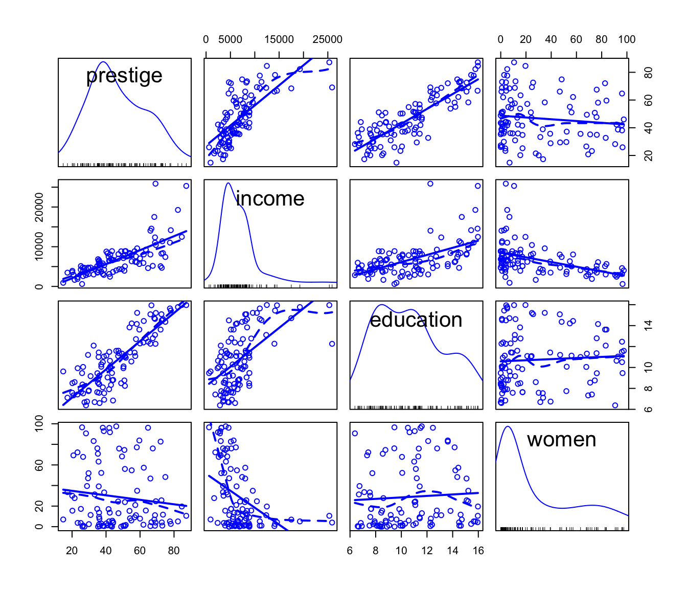
Scatterplot matrix for the Prestige data.

The powerTransform() function in the car package transforms variables towards multivariate normality by a generalization of Box and Cox’s maximum-likelihood-like approach (Box & Cox, 1964). Several “families” of power transformations can be used, including the original Box-Cox family, simple powers (and roots), and two adaptations of the Box-Cox family to data that may include negative values and zeros: the Box-Cox-with-negatives family and the Yeo-Johnson family; see Weisberg (2014, Chapter 8), and Fox & Weisberg (2019, Chapter 3) for details. Because women has some zero values, we use the Yeo-Johnson family:

trans <- powerTransform(cbind(income, education, women) ~ 1,
                        data = Prestige,
                        family = "yjPower")
summary(trans)
#> yjPower Transformations to Multinormality 
#>           Est Power Rounded Pwr Wald Lwr Bnd Wald Upr Bnd
#> income       0.2678        0.33       0.1051       0.4304
#> education    0.5162        1.00      -0.2822       1.3145
#> women        0.1630        0.16       0.0112       0.3149
#> 
#>  Likelihood ratio test that all transformation parameters are equal to 0
#>                              LRT df    pval
#> LR test, lambda = (0 0 0) 15.739  3 0.00128

We thus have evidence of the desirability of transforming income (by the $1/3$ power) and women (by the $0.16$ power—which is close to the “0” power, i.e., the log transformation), but not education. Applying the “rounded” power transformations makes the predictors better-behaved:

P <- Prestige[, c("prestige", "income", "education", "women")]
(lambdas <- trans$roundlam)
#>    income education     women 
#>   0.33000   1.00000   0.16302
names(lambdas) <- c("income", "education", "women")
for (var in c("income", "education", "women")) {
  P[, var] <- yjPower(P[, var], lambda = lambdas[var])
}
summary(P)
#>     prestige        income       education         women     
#>  Min.   :14.8   Min.   :22.2   Min.   : 6.38   Min.   :0.00  
#>  1st Qu.:35.2   1st Qu.:44.2   1st Qu.: 8.45   1st Qu.:1.73  
#>  Median :43.6   Median :50.3   Median :10.54   Median :3.36  
#>  Mean   :46.8   Mean   :50.8   Mean   :10.74   Mean   :3.50  
#>  3rd Qu.:59.3   3rd Qu.:56.2   3rd Qu.:12.65   3rd Qu.:5.59  
#>  Max.   :87.2   Max.   :83.6   Max.   :15.97   Max.   :6.83

scatterplotMatrix(
  ~ prestige + income + education + women,
  data = P,
  smooth = list(spread = FALSE)
)

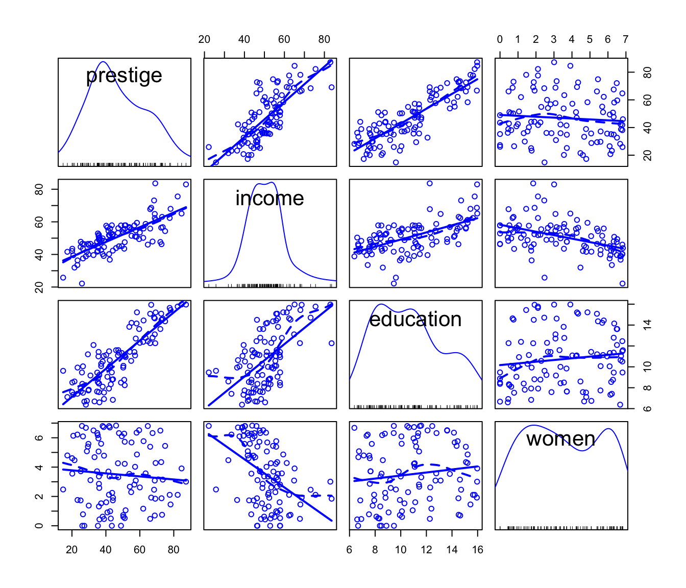
Scatterplot matrix for the Prestige data with the predictors transformed.

Comparing the MSE for the regressions with the original and transformed predictors shows a advantage to the latter:

m.pres <- lm(prestige ~ income + education + women, data = Prestige)
m.pres.trans <- lm(prestige ~ income + education + women, data = P)
mse(Prestige$prestige, fitted(m.pres))
#> [1] 59.153
#> attr(,"casewise loss")
#> [1] "(y - yhat)^2"
mse(P$prestige, fitted(m.pres.trans))
#> [1] 50.6
#> attr(,"casewise loss")
#> [1] "(y - yhat)^2"

Similarly, component+residual plots for the two regressions, produced by the crPlots() function in the car package, suggest that the partial relationship of prestige to income is more nearly linear in the transformed data, but the transformation of women fails to capture what appears to be a slight quadratic partial relationship; the partial relationship of prestige to education is close to linear in both regressions:

crPlots(m.pres)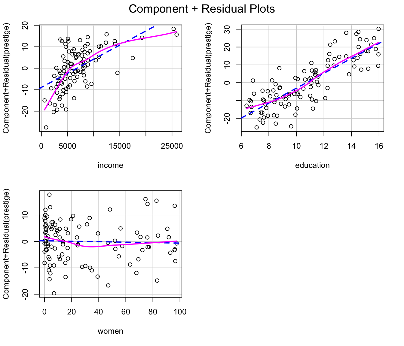

Component+residual plots for the Prestige regression with the original predictors.

crPlots(m.pres.trans)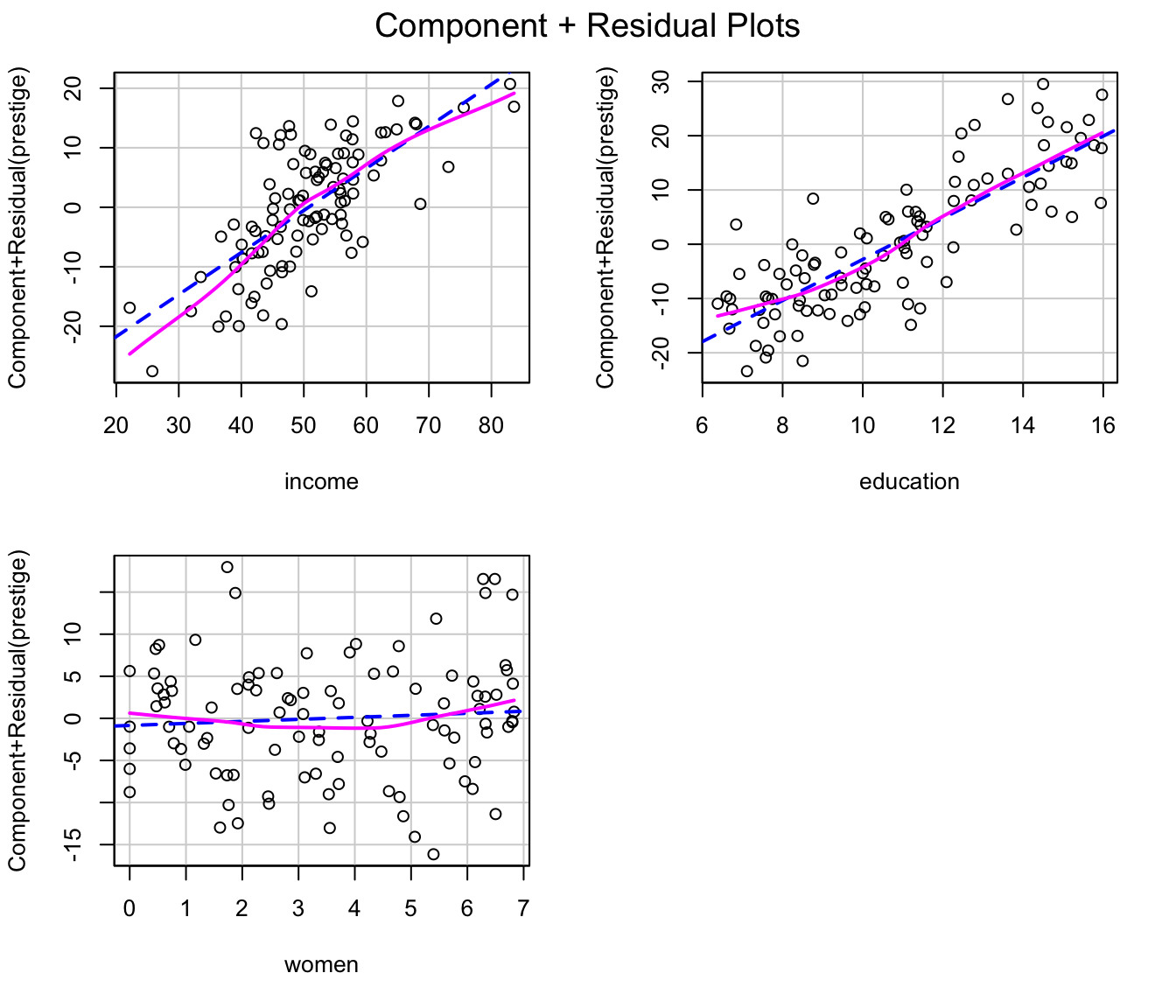

Component+residual plots for the Prestige regression with transformed predictors.

Having transformed the predictors towards multinormality, we now consider whether there’s evidence for transforming the response (using powerTransform() for Box and Cox’s original method), and we discover that there’s not:

summary(powerTransform(m.pres.trans))
#> bcPower Transformation to Normality 
#>    Est Power Rounded Pwr Wald Lwr Bnd Wald Upr Bnd
#> Y1    1.0194           1       0.6773       1.3615
#> 
#> Likelihood ratio test that transformation parameter is equal to 0
#>  (log transformation)
#>                          LRT df     pval
#> LR test, lambda = (0) 32.217  1 1.38e-08
#> 
#> Likelihood ratio test that no transformation is needed
#>                            LRT df  pval
#> LR test, lambda = (1) 0.012384  1 0.911

The selectTrans() function in the cv package automates the process of selecting predictor and response transformations. The function takes a data set and “working” model as arguments, along with the candidate predictors and response for transformation, and the transformation family to employ. If the predictors argument is missing then only the response is transformed, and if the response argument is missing, only the supplied predictors are transformed. The default family for transforming the predictors is "bcPower"—the original Box-Cox family—as is the default family.y for transforming the response; here we specify family="yjPower because of the zeros in women. selectTrans() returns the result of applying a lack-of-fit criterion to the model after the selected transformation is applied, with the default criterion=mse:

selectTrans(
  data = Prestige,
  model = m.pres,
  predictors = c("income", "education", "women"),
  response = "prestige",
  family = "yjPower"
)
#> $criterion
#> [1] 50.6
#> attr(,"casewise loss")
#> [1] "(y - yhat)^2"
#> 
#> $model
#> NULL

selectTrans() also takes an optional indices argument, making it suitable for doing computations on a subset of the data (i.e., a CV fold), and hence for use with cv() (see ?selectTrans for details):

cvs <- cv(
  selectTrans,
  data = Prestige,
  working.model = m.pres,
  seed = 1463,
  predictors = c("income", "education", "women"),
  response = "prestige",
  family = "yjPower"
)
#> R RNG seed set to 1463
summary(cvs)
#> 10-Fold Cross Validation
#> criterion: mse
#> cross-validation criterion = 54.487
#> bias-adjusted cross-validation criterion = 54.308
#> full-sample criterion = 50.6

cv(m.pres, seed = 1463) # untransformed model with same folds
#> R RNG seed set to 1463
#> cross-validation criterion (mse) = 63.293

compareFolds(cvs)
#> CV criterion by folds:
#>  fold.1  fold.2  fold.3  fold.4  fold.5  fold.6  fold.7  fold.8  fold.9 fold.10 
#>  63.453  79.257  20.634  94.569  19.902  55.821  26.555  75.389  55.702  50.215 
#> 
#> Coefficients by folds:
#>         lam.education lam.income lam.women lambda
#> Fold 1          1.000      0.330     0.330      1
#> Fold 2          1.000      0.330     0.169      1
#> Fold 3          1.000      0.330     0.330      1
#> Fold 4          1.000      0.330     0.330      1
#> Fold 5          1.000      0.330     0.000      1
#> Fold 6          1.000      0.330     0.330      1
#> Fold 7          1.000      0.330     0.330      1
#> Fold 8          1.000      0.330     0.000      1
#> Fold 9          1.000      0.330     0.000      1
#> Fold 10         1.000      0.330     0.000      1

The results suggest that the predictive power of the transformed regression is reliably greater than that of the untransformed regression (though in both case, the cross-validated MSE is considerably higher than the MSE computed for the whole data). Examining the selected transformations for each fold reveals that the predictor education and the response prestige are never transformed; that the $1/3$ power is selected for income in all of the folds; and that the transformation selected for women varies narrowly across the folds between the $0$th power (i.e., log) and the $1/3$ power.

Selecting both transformations and predictors²

As we mentioned, Hastie et al. (2009, sec. 7.10.2: “The Wrong and Right Way to Do Cross-validation”) explain that honest cross-validation has to take account of model specification and selection. Statistical modeling is at least partly a craft, and one could imagine applying that craft to successive partial data sets, each with a fold removed. The resulting procedure would be tedious, though possibly worth the effort, but it would also be difficult to realize in practice: After all, we can hardly erase our memory of statistical modeling choices between analyzing partial data sets.

Alternatively, if we’re able to automate the process of model selection, then we can more realistically apply CV mechanically. That’s what we did in the preceding two sections, first for predictor selection and then for selection of transformations in regression. In this section, we consider the case where we both select variable transformations and then proceed to select predictors. It’s insufficient to apply these steps sequentially, first, for example, using cv() with selectTrans() and then with selectStepAIC(); rather we should apply the whole model-selection procedure with each fold omitted. The selectTransAndStepAIC() function, also supplied by the cv package, does exactly that.

To illustrate this process, we return to the Auto data set:

summary(Auto)
#>       mpg         cylinders     displacement   horsepower        weight    
#>  Min.   : 9.0   Min.   :3.00   Min.   : 68   Min.   : 46.0   Min.   :1613  
#>  1st Qu.:17.0   1st Qu.:4.00   1st Qu.:105   1st Qu.: 75.0   1st Qu.:2225  
#>  Median :22.8   Median :4.00   Median :151   Median : 93.5   Median :2804  
#>  Mean   :23.4   Mean   :5.47   Mean   :194   Mean   :104.5   Mean   :2978  
#>  3rd Qu.:29.0   3rd Qu.:8.00   3rd Qu.:276   3rd Qu.:126.0   3rd Qu.:3615  
#>  Max.   :46.6   Max.   :8.00   Max.   :455   Max.   :230.0   Max.   :5140  
#>                                                                            
#>   acceleration       year        origin                     name    
#>  Min.   : 8.0   Min.   :70   Min.   :1.00   amc matador       :  5  
#>  1st Qu.:13.8   1st Qu.:73   1st Qu.:1.00   ford pinto        :  5  
#>  Median :15.5   Median :76   Median :1.00   toyota corolla    :  5  
#>  Mean   :15.5   Mean   :76   Mean   :1.58   amc gremlin       :  4  
#>  3rd Qu.:17.0   3rd Qu.:79   3rd Qu.:2.00   amc hornet        :  4  
#>  Max.   :24.8   Max.   :82   Max.   :3.00   chevrolet chevette:  4  
#>                                             (Other)           :365
xtabs( ~ year, data = Auto)
#> year
#> 70 71 72 73 74 75 76 77 78 79 80 81 82 
#> 29 27 28 40 26 30 34 28 36 29 27 28 30
xtabs( ~ origin, data = Auto)
#> origin
#>   1   2   3 
#> 245  68  79
xtabs( ~ cylinders, data = Auto)
#> cylinders
#>   3   4   5   6   8 
#>   4 199   3  83 103

We previously used the Auto here in a preliminary example where we employed CV to inform the selection of the order of a polynomial regression of mpg on horsepower. Here, we consider more generally the problem of predicting mpg from the other variables in the Auto data. We begin with a bit of data management, and then examine the pairwise relationships among the numeric variables in the data set:

Auto$cylinders <- factor(Auto$cylinders,
                         labels = c("3.4", "3.4", "5.6", "5.6", "8"))
Auto$year <- as.factor(Auto$year)
Auto$origin <- factor(Auto$origin,
                      labels = c("America", "Europe", "Japan"))
rownames(Auto) <- make.names(Auto$name, unique = TRUE)
Auto$name <- NULL

scatterplotMatrix(
  ~ mpg + displacement + horsepower + weight + acceleration,
  smooth = list(spread = FALSE),
  data = Auto
)

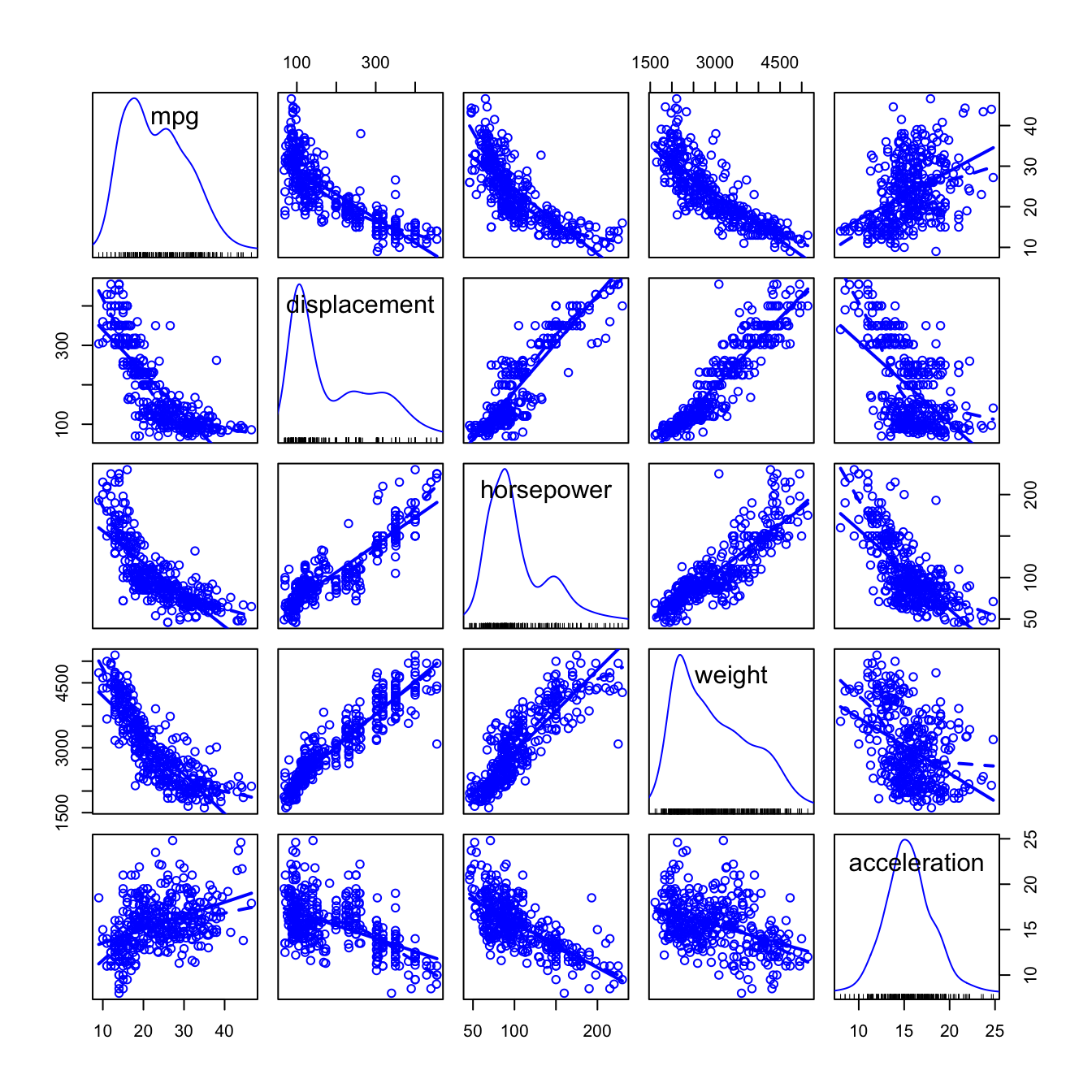
Scatterplot matrix for the numeric variables in the Auto data

A comment before we proceed: origin is clearly categorical and so converting it to a factor is natural, but we could imagine treating cylinders and year as numeric predictors. There are, however, only 5 distinct values of cylinders (ranging from 3 to 8), but cars with 3 or 5 cylinders are rare. and none of the cars has 7 cylinders. There are similarly only 13 distinct years between 1970 and 1982 in the data, and the relationship between mpg and year is difficult to characterize.³ It’s apparent that most these variables are positively skewed and that many of the pairwise relationships among them are nonlinear.

We begin with a “working model” that specifies linear partial relationships of the response to the numeric predictors:

m.auto <- lm(mpg ~ ., data = Auto)
summary(m.auto)
#> 
#> Call:
#> lm(formula = mpg ~ ., data = Auto)
#> 
#> Residuals:
#>    Min     1Q Median     3Q    Max 
#> -9.006 -1.745 -0.092  1.525 10.950 
#> 
#> Coefficients:
#>               Estimate Std. Error t value Pr(>|t|)    
#> (Intercept)  37.034132   1.969393   18.80  < 2e-16 ***
#> cylinders5.6 -2.602941   0.655200   -3.97  8.5e-05 ***
#> cylinders8   -0.582458   1.171452   -0.50  0.61934    
#> displacement  0.017425   0.006734    2.59  0.01004 *  
#> horsepower   -0.041353   0.013379   -3.09  0.00215 ** 
#> weight       -0.005548   0.000632   -8.77  < 2e-16 ***
#> acceleration  0.061527   0.088313    0.70  0.48643    
#> year71        0.968058   0.837390    1.16  0.24841    
#> year72       -0.601435   0.825115   -0.73  0.46652    
#> year73       -0.687689   0.740272   -0.93  0.35351    
#> year74        1.375576   0.876500    1.57  0.11741    
#> year75        0.929929   0.859072    1.08  0.27974    
#> year76        1.559893   0.822505    1.90  0.05867 .  
#> year77        2.909416   0.841729    3.46  0.00061 ***
#> year78        3.175198   0.798940    3.97  8.5e-05 ***
#> year79        5.019299   0.845759    5.93  6.8e-09 ***
#> year80        9.099763   0.897293   10.14  < 2e-16 ***
#> year81        6.688660   0.885218    7.56  3.3e-13 ***
#> year82        8.071125   0.870668    9.27  < 2e-16 ***
#> originEurope  2.046664   0.517124    3.96  9.1e-05 ***
#> originJapan   2.144887   0.507717    4.22  3.0e-05 ***
#> ---
#> Signif. codes:  0 '***' 0.001 '**' 0.01 '*' 0.05 '.' 0.1 ' ' 1
#> 
#> Residual standard error: 2.92 on 371 degrees of freedom
#> Multiple R-squared:  0.867,  Adjusted R-squared:  0.86 
#> F-statistic:  121 on 20 and 371 DF,  p-value: <2e-16

Anova(m.auto)
#> Anova Table (Type II tests)
#> 
#> Response: mpg
#>              Sum Sq  Df F value  Pr(>F)    
#> cylinders       292   2   17.09 7.9e-08 ***
#> displacement     57   1    6.70  0.0100 *  
#> horsepower       82   1    9.55  0.0021 ** 
#> weight          658   1   76.98 < 2e-16 ***
#> acceleration      4   1    0.49  0.4864    
#> year           3017  12   29.40 < 2e-16 ***
#> origin          190   2   11.13 2.0e-05 ***
#> Residuals      3173 371                    
#> ---
#> Signif. codes:  0 '***' 0.001 '**' 0.01 '*' 0.05 '.' 0.1 ' ' 1

crPlots(m.auto)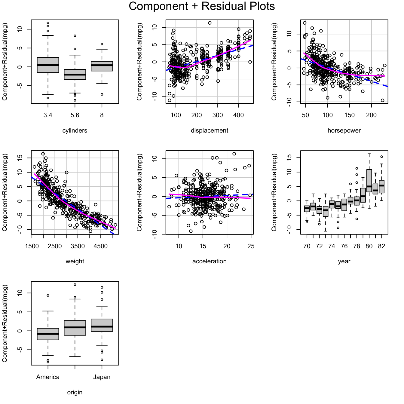

Component+residual plots for the working model fit to the Auto data

The component+residual plots, created with the crPlots() function in the previously loaded car package, clearly reveal the inadequacy of the model.

We proceed to transform the numeric predictors towards multi-normality:

num.predictors <-
  c("displacement", "horsepower", "weight", "acceleration")
tr.x <- powerTransform(Auto[, num.predictors])
summary(tr.x)
#> bcPower Transformations to Multinormality 
#>              Est Power Rounded Pwr Wald Lwr Bnd Wald Upr Bnd
#> displacement   -0.0509           0      -0.2082       0.1065
#> horsepower     -0.1249           0      -0.2693       0.0194
#> weight         -0.0870           0      -0.2948       0.1208
#> acceleration    0.3061           0      -0.0255       0.6376
#> 
#> Likelihood ratio test that transformation parameters are equal to 0
#>  (all log transformations)
#>                                LRT df  pval
#> LR test, lambda = (0 0 0 0) 4.8729  4 0.301
#> 
#> Likelihood ratio test that no transformations are needed
#>                                LRT df   pval
#> LR test, lambda = (1 1 1 1) 390.08  4 <2e-16

We then apply the (rounded) transformations—all, as it turns out, logs—to the data and re-estimate the model:

A <- Auto
powers <- tr.x$roundlam
for (pred in num.predictors) {
  A[, pred] <- bcPower(A[, pred], lambda = powers[pred])
}
head(A)
#>                           mpg cylinders displacement horsepower weight
#> chevrolet.chevelle.malibu  18         8       5.7268     4.8675 8.1617
#> buick.skylark.320          15         8       5.8579     5.1059 8.2142
#> plymouth.satellite         18         8       5.7621     5.0106 8.1421
#> amc.rebel.sst              16         8       5.7170     5.0106 8.1412
#> ford.torino                17         8       5.7104     4.9416 8.1458
#> ford.galaxie.500           15         8       6.0615     5.2883 8.3759
#>                           acceleration year  origin
#> chevrolet.chevelle.malibu       2.4849   70 America
#> buick.skylark.320               2.4423   70 America
#> plymouth.satellite              2.3979   70 America
#> amc.rebel.sst                   2.4849   70 America
#> ford.torino                     2.3514   70 America
#> ford.galaxie.500                2.3026   70 America

m <- update(m.auto, data = A)

Finally, we perform Box-Cox regression to transform the response (also obtaining a log transformation):

summary(powerTransform(m))
#> bcPower Transformation to Normality 
#>    Est Power Rounded Pwr Wald Lwr Bnd Wald Upr Bnd
#> Y1    0.0024           0      -0.1607       0.1654
#> 
#> Likelihood ratio test that transformation parameter is equal to 0
#>  (log transformation)
#>                              LRT df  pval
#> LR test, lambda = (0) 0.00080154  1 0.977
#> 
#> Likelihood ratio test that no transformation is needed
#>                          LRT df   pval
#> LR test, lambda = (1) 124.13  1 <2e-16

m <- update(m, log(mpg) ~ .)
summary(m)
#> 
#> Call:
#> lm(formula = log(mpg) ~ cylinders + displacement + horsepower + 
#>     weight + acceleration + year + origin, data = A)
#> 
#> Residuals:
#>     Min      1Q  Median      3Q     Max 
#> -0.3341 -0.0577  0.0041  0.0607  0.3808 
#> 
#> Coefficients:
#>              Estimate Std. Error t value Pr(>|t|)    
#> (Intercept)    8.8965     0.3582   24.84  < 2e-16 ***
#> cylinders5.6  -0.0636     0.0257   -2.47    0.014 *  
#> cylinders8    -0.0769     0.0390   -1.97    0.049 *  
#> displacement   0.0280     0.0515    0.54    0.587    
#> horsepower    -0.2901     0.0563   -5.15  4.2e-07 ***
#> weight        -0.5427     0.0819   -6.62  1.2e-10 ***
#> acceleration  -0.1421     0.0563   -2.52    0.012 *  
#> year71         0.0250     0.0289    0.87    0.387    
#> year72        -0.0168     0.0289   -0.58    0.562    
#> year73        -0.0426     0.0260   -1.64    0.103    
#> year74         0.0493     0.0304    1.62    0.106    
#> year75         0.0472     0.0296    1.59    0.112    
#> year76         0.0709     0.0284    2.49    0.013 *  
#> year77         0.1324     0.0293    4.52  8.2e-06 ***
#> year78         0.1447     0.0278    5.21  3.1e-07 ***
#> year79         0.2335     0.0292    7.99  1.7e-14 ***
#> year80         0.3238     0.0317   10.22  < 2e-16 ***
#> year81         0.2565     0.0309    8.29  2.1e-15 ***
#> year82         0.3076     0.0304   10.13  < 2e-16 ***
#> originEurope   0.0492     0.0195    2.52    0.012 *  
#> originJapan    0.0441     0.0195    2.26    0.024 *  
#> ---
#> Signif. codes:  0 '***' 0.001 '**' 0.01 '*' 0.05 '.' 0.1 ' ' 1
#> 
#> Residual standard error: 0.104 on 371 degrees of freedom
#> Multiple R-squared:  0.911,  Adjusted R-squared:  0.906 
#> F-statistic:  189 on 20 and 371 DF,  p-value: <2e-16

Anova(m)
#> Anova Table (Type II tests)
#> 
#> Response: log(mpg)
#>              Sum Sq  Df F value  Pr(>F)    
#> cylinders      0.07   2    3.05   0.048 *  
#> displacement   0.00   1    0.30   0.587    
#> horsepower     0.29   1   26.54 4.2e-07 ***
#> weight         0.48   1   43.88 1.2e-10 ***
#> acceleration   0.07   1    6.37   0.012 *  
#> year           4.45  12   34.13 < 2e-16 ***
#> origin         0.08   2    3.71   0.025 *  
#> Residuals      4.03 371                    
#> ---
#> Signif. codes:  0 '***' 0.001 '**' 0.01 '*' 0.05 '.' 0.1 ' ' 1

The transformed numeric variables are much better-behaved:

scatterplotMatrix(
  ~ log(mpg) + displacement + horsepower + weight
  + acceleration,
  smooth = list(spread = FALSE),
  data = A
)

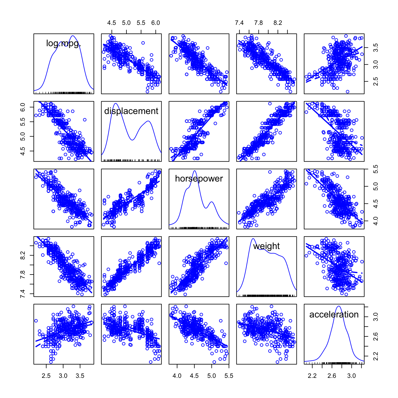
Scatterplot matrix for the transformed numeric variables in the Auto data

And the partial relationships in the model fit to the transformed data are much more nearly linear:

crPlots(m)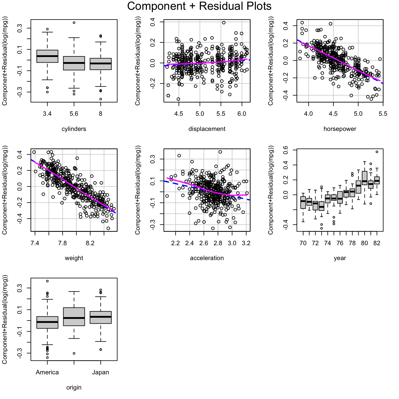

Component+residual plots for the model fit to the transformed Auto data

Having transformed both the numeric predictors and the response, we proceed to use the stepAIC() function in the MASS package to perform predictor selection, employing the BIC model-selection criterion (by setting the k argument of stepAIC() to $\log(n)$):

m.step <- stepAIC(m, k=log(nrow(A)), trace=FALSE)
summary(m.step)
#> 
#> Call:
#> lm(formula = log(mpg) ~ horsepower + weight + acceleration + 
#>     year + origin, data = A)
#> 
#> Residuals:
#>     Min      1Q  Median      3Q     Max 
#> -0.3523 -0.0568  0.0068  0.0674  0.3586 
#> 
#> Coefficients:
#>              Estimate Std. Error t value Pr(>|t|)    
#> (Intercept)   9.43459    0.26153   36.07  < 2e-16 ***
#> horsepower   -0.27625    0.05614   -4.92  1.3e-06 ***
#> weight       -0.60907    0.05600  -10.88  < 2e-16 ***
#> acceleration -0.13138    0.05319   -2.47  0.01397 *  
#> year71        0.02798    0.02894    0.97  0.33412    
#> year72       -0.00711    0.02845   -0.25  0.80274    
#> year73       -0.03953    0.02601   -1.52  0.12947    
#> year74        0.05275    0.02999    1.76  0.07936 .  
#> year75        0.05320    0.02928    1.82  0.07004 .  
#> year76        0.07432    0.02821    2.63  0.00878 ** 
#> year77        0.13793    0.02888    4.78  2.6e-06 ***
#> year78        0.14588    0.02753    5.30  2.0e-07 ***
#> year79        0.23604    0.02908    8.12  7.0e-15 ***
#> year80        0.33527    0.03115   10.76  < 2e-16 ***
#> year81        0.26287    0.03056    8.60  < 2e-16 ***
#> year82        0.32339    0.02961   10.92  < 2e-16 ***
#> originEurope  0.05582    0.01678    3.33  0.00097 ***
#> originJapan   0.04355    0.01748    2.49  0.01314 *  
#> ---
#> Signif. codes:  0 '***' 0.001 '**' 0.01 '*' 0.05 '.' 0.1 ' ' 1
#> 
#> Residual standard error: 0.105 on 374 degrees of freedom
#> Multiple R-squared:  0.909,  Adjusted R-squared:  0.905 
#> F-statistic:  220 on 17 and 374 DF,  p-value: <2e-16

Anova(m.step)
#> Anova Table (Type II tests)
#> 
#> Response: log(mpg)
#>              Sum Sq  Df F value  Pr(>F)    
#> horsepower     0.27   1   24.21 1.3e-06 ***
#> weight         1.30   1  118.28 < 2e-16 ***
#> acceleration   0.07   1    6.10  0.0140 *  
#> year           4.76  12   36.05 < 2e-16 ***
#> origin         0.14   2    6.21  0.0022 ** 
#> Residuals      4.11 374                    
#> ---
#> Signif. codes:  0 '***' 0.001 '**' 0.01 '*' 0.05 '.' 0.1 ' ' 1

The selected model includes three of the numeric predictors, horsepower, weight, and acceleration, along with the factors year and origin. We can calculate the MSE for this model, but we expect that the result will be optimistic because we used the whole data to help specify the model

mse(Auto$mpg, exp(fitted(m.step)))
#> [1] 6.5121
#> attr(,"casewise loss")
#> [1] "(y - yhat)^2"

This is considerably smaller than the MSE for the original working model:

mse(Auto$mpg, fitted(m.auto))
#> [1] 8.0932
#> attr(,"casewise loss")
#> [1] "(y - yhat)^2"

A perhaps subtle point is that we compute the MSE for the selected model on the original mpg response scale rather than the log scale, so as to make the selected model comparable to the working model. That’s slightly uncomfortable given the skewed distribution of mpg. An alternative is to use the median absolute error instead of the mean-squared error, employing the medAbsErr() function from the cv package:

medAbsErr(Auto$mpg, exp(fitted(m.step)))
#> [1] 1.3396
medAbsErr(Auto$mpg, fitted(m.auto))
#> [1] 1.6661

Now let’s use cv() with selectTransAndStepAIC() to automate and cross-validate the whole model-specification process:

num.predictors
#> [1] "displacement" "horsepower"   "weight"       "acceleration"
cvs <- cv(
  selectTransStepAIC,
  data = Auto,
  seed = 76692,
  working.model = m.auto,
  predictors = num.predictors,
  response = "mpg",
  AIC = FALSE,
  criterion = medAbsErr
)
#> R RNG seed set to 76692
summary(cvs)
#> 10-Fold Cross Validation
#> criterion: medAbsErr
#> cross-validation criterion = 1.4951
#> full-sample criterion = 1.3396

compareFolds(cvs)
#> CV criterion by folds:
#>  fold.1  fold.2  fold.3  fold.4  fold.5  fold.6  fold.7  fold.8  fold.9 fold.10 
#>  1.5639  1.5766  1.3698  1.2381  1.2461  1.5826  1.3426  1.1905  1.1355  1.5854 
#> 
#> Coefficients by folds:
#>         (Intercept) horsepower lam.acceleration lam.displacement lam.horsepower
#> Fold 1      9.71384   -0.17408          0.50000          0.00000        0.00000
#> Fold 2      9.21713   -0.31480          0.00000          0.00000        0.00000
#> Fold 3      9.61824   -0.19248          0.00000          0.00000        0.00000
#> Fold 4      8.69910   -0.25523          0.50000          0.00000        0.00000
#> Fold 5      9.14403   -0.14934          0.00000          0.00000        0.00000
#> Fold 6      9.63481   -0.16739          0.50000          0.00000        0.00000
#> Fold 7      9.98933   -0.36847          0.00000          0.00000       -0.15447
#> Fold 8      9.06301   -0.29721          0.00000          0.00000        0.00000
#> Fold 9      8.88315   -0.22684          0.00000          0.00000        0.00000
#> Fold 10     9.61727   -0.17086          0.00000          0.00000        0.00000
#>         lam.weight   lambda   weight   year71   year72   year73   year74
#> Fold 1     0.00000  0.00000 -0.74636  0.03764 -0.00327 -0.02477  0.05606
#> Fold 2     0.00000  0.00000 -0.47728  0.02173 -0.01488 -0.03770  0.04312
#> Fold 3     0.00000  0.00000 -0.72085  0.01128 -0.02569 -0.03872  0.05187
#> Fold 4     0.00000  0.00000 -0.53846  0.02153 -0.02922 -0.05181  0.04136
#> Fold 5     0.00000  0.00000 -0.69081  0.02531 -0.01062 -0.04625  0.05039
#> Fold 6     0.00000  0.00000 -0.74049  0.02456  0.00759 -0.03412  0.06266
#> Fold 7     0.00000  0.00000 -0.72843  0.02532 -0.01271 -0.04144  0.04568
#> Fold 8     0.00000  0.00000 -0.46392  0.02702 -0.02041 -0.05605  0.04437
#> Fold 9     0.00000  0.00000 -0.47136  0.00860 -0.03620 -0.04835  0.01906
#> Fold 10    0.00000  0.00000 -0.73550  0.02937 -0.00899 -0.03814  0.05408
#>           year75   year76   year77   year78   year79   year80   year81   year82
#> Fold 1   0.07080  0.07250  0.14420  0.14281  0.23266  0.35127  0.25635  0.30546
#> Fold 2   0.04031  0.06718  0.13094  0.14917  0.21871  0.33192  0.26196  0.30943
#> Fold 3   0.03837  0.06399  0.11593  0.12601  0.20499  0.32821  0.24478  0.29204
#> Fold 4   0.04072  0.05537  0.12292  0.14083  0.22878  0.32947  0.25140  0.27248
#> Fold 5   0.05596  0.07044  0.13356  0.14724  0.24675  0.33331  0.26938  0.32594
#> Fold 6   0.06940  0.07769  0.14211  0.14647  0.23532  0.34761  0.26737  0.33062
#> Fold 7   0.03614  0.07385  0.12976  0.14040  0.23976  0.33998  0.27652  0.30659
#> Fold 8   0.06573  0.08135  0.13158  0.13987  0.23011  0.32880  0.25886  0.30538
#> Fold 9   0.03018  0.05846  0.10536  0.11722  0.20665  0.31533  0.23352  0.29375
#> Fold 10  0.04881  0.07862  0.14101  0.14313  0.23258  0.35649  0.26214  0.32421
#>         acceleration displacement cylinders5.6 cylinders8 originEurope
#> Fold 1                                                                
#> Fold 2      -0.18909     -0.09197                                     
#> Fold 3                                                                
#> Fold 4      -0.03484                  -0.09080   -0.10909             
#> Fold 5                                                         0.06261
#> Fold 6                                                                
#> Fold 7                                                                
#> Fold 8      -0.17676     -0.10542                                     
#> Fold 9      -0.14514     -0.13452                                     
#> Fold 10                                                               
#>         originJapan
#> Fold 1             
#> Fold 2             
#> Fold 3             
#> Fold 4             
#> Fold 5         0.04
#> Fold 6             
#> Fold 7             
#> Fold 8             
#> Fold 9             
#> Fold 10

Here, as for selectTrans(), the predictors and response arguments specify candidate variables for transformation, and AIC=FALSE uses the BIC for model selection. The starting model, m.auto, is the working model fit to the Auto data. The CV criterion isn’t bias-adjusted because median absolute error isn’t a mean of casewise error components.

Some noteworthy points:

• selectTransStepAIC() automatically computes CV cost criteria, here the median absolute error, on the untransformed response scale.
• The estimate of the median absolute error that we obtain by cross-validating the whole model-specification process is a little larger than the median absolute error computed for the model we fit to the Auto data separately selecting transformations of the predictors and the response and then selecting predictors for the whole data set.
• When we look at the transformations and predictors selected with each of the 10 folds omitted (i.e., the output of compareFolds()), we see that there is little uncertainty in choosing variable transformations (the lam.*s for the $x$s and lambda for $y$ in the output), but considerably more uncertainty in subsequently selecting predictors: horsepower, weight, and year are always included among the selected predictors; acceleration and displacement are each included respectively in 4 and 3 of 10 selected models; and cylinders and origin are each included in only 1 of 10 models. Recall that when we selected predictors for the full data, we obtained a model with horsepower, weight, acceleration, year, and origin.

References

Box, G. E. P., & Cox, D. R. (1964). An analysis of transformations. Journal of the Royal Statistical Society, Series B, 26, 211–252.

Fox, J., & Weisberg, S. (2019). An R companion to applied regression (Third edition). Thousand Oaks CA: Sage.

Hastie, T., Tibshirani, R., & Friedman, J. (2009). The elements of statistical learning: Data mining, inference, and prediction (Second edition). New York: Springer. Retrieved from https://hastie.su.domains/ElemStatLearn/printings/ESLII_print12_toc.pdf

James, G., Witten, D., Hastie, T., & Tibshirani, R. (2021). An introduction to statistical learning with applications in R (Second edition). New York: Springer.

Venables, W. N., & Ripley, B. D. (2002). Modern applied statistics with S (Fourth edition). New York: Springer.

Weisberg, S. (2014). Applied linear regression (Second edition). Hoboken NJ: Wiley.