Cross-validating regression models

Introduction to the cv package

John Fox and Georges Monette

2024-10-04

This vignette covers the basics of using the cv package for cross-validation. The first, and major, section of the vignette consists of examples that fit linear and generalized linear models to data sets with independently sampled cases. Brief sections follow on replicating cross-validation, manipulating the objects produced by cv() and related functions, and employing parallel computations.

There are several other vignettes associated with the cv package: on cross-validating mixed-effects models; on cross-validating model-selection procedures; and on technical details, such as computational procedures.

Cross-validation

Cross-validation (CV) is an essentially simple and intuitively reasonable approach to estimating the predictive accuracy of regression models. CV is developed in many standard sources on regression modeling and “machine learning”—we particularly recommend James, Witten, Hastie, & Tibshirani (2021, secs. 5.1, 5.3)—and so we will describe the method only briefly here before taking up computational issues and some examples. See Arlot & Celisse (2010) for a wide-ranging, if technical, survey of cross-validation and related methods that emphasizes the statistical properties of CV.

Validating research by replication on independently collected data is a common scientific norm. Emulating this process in a single study by data-division is less common: The data are randomly divided into two, possibly equal-size, parts; the first part is used to develop and fit a statistical model; and then the second part is used to assess the adequacy of the model fit to the first part of the data. Data-division, however, suffers from two problems: (1) Dividing the data decreases the sample size and thus increases sampling error; and (2), even more disconcertingly, particularly in smaller samples, the results can vary substantially based on the random division of the data: See Harrell (2015, sec. 5.3) for this and other remarks about data-division and cross-validation.

Cross-validation speaks to both of these issues. In CV, the data are randomly divided as equally as possible into several, say $k$, parts, called “folds.” The statistical model is fit $k$ times, leaving each fold out in turn. Each fitted model is then used to predict the response variable for the cases in the omitted fold. A CV criterion or “cost” measure, such as the mean-squared error (“MSE”) of prediction, is then computed using these predicted values. In the extreme $k = n$, the number of cases in the data, thus omitting individual cases and refitting the model $n$ times—a procedure termed “leave-one-out (LOO) cross-validation.”

Because the $n$ models are each fit to $n - 1$ cases, LOO CV produces a nearly unbiased estimate of prediction error. The $n$ regression models are highly statistically dependent, however, based as they are on nearly the same data, and so the resulting estimate of prediction error has larger variance than if the predictions from the models fit to the $n$ data sets were independent.

Because predictions are based on smaller data sets, each of size approximately $n - n/k$, estimated prediction error for $k$-fold CV with $k = 5$ or $10$ (commonly employed choices) is more biased than estimated prediction error for LOO CV. It is possible, however, to correct $k$-fold CV for bias (see below).

The relative variance of prediction error for LOO CV and $k$-fold CV (with $k < n$) is more complicated: Because the overlap between the data sets with each fold omitted is smaller for $k$-fold CV than for LOO CV, the dependencies among the predictions are smaller for the former than for the latter, tending to produce smaller variance in prediction error for $k$-fold CV. In contrast, there are factors that tend to inflate the variance of prediction error in $k$-fold CV, including the reduced size of the data sets with each fold omitted and the randomness induced by the selection of folds—in LOO CV the folds are not random.

Examples

Polynomial regression for the Auto data

The data for this example are drawn from the ISLR2 package for R, associated with James et al. (2021). The presentation here is close (though not identical) to that in the original source (James et al., 2021, secs. 5.1, 5.3), and it demonstrates the use of the cv() function in the cv package.¹

The Auto dataset contains information about 392 cars:

data("Auto", package="ISLR2")
head(Auto)
#>   mpg cylinders displacement horsepower weight acceleration year origin
#> 1  18         8          307        130   3504         12.0   70      1
#> 2  15         8          350        165   3693         11.5   70      1
#> 3  18         8          318        150   3436         11.0   70      1
#> 4  16         8          304        150   3433         12.0   70      1
#> 5  17         8          302        140   3449         10.5   70      1
#> 6  15         8          429        198   4341         10.0   70      1
#>                        name
#> 1 chevrolet chevelle malibu
#> 2         buick skylark 320
#> 3        plymouth satellite
#> 4             amc rebel sst
#> 5               ford torino
#> 6          ford galaxie 500
dim(Auto)
#> [1] 392   9

With the exception of origin (which we don’t use here), these variables are largely self-explanatory, except possibly for units of measurement: for details see help("Auto", package="ISLR2").

We’ll focus here on the relationship of mpg (miles per gallon) to horsepower, as displayed in the following scatterplot:

plot(mpg ~ horsepower, data=Auto)

mpg vs horsepower for the Auto data

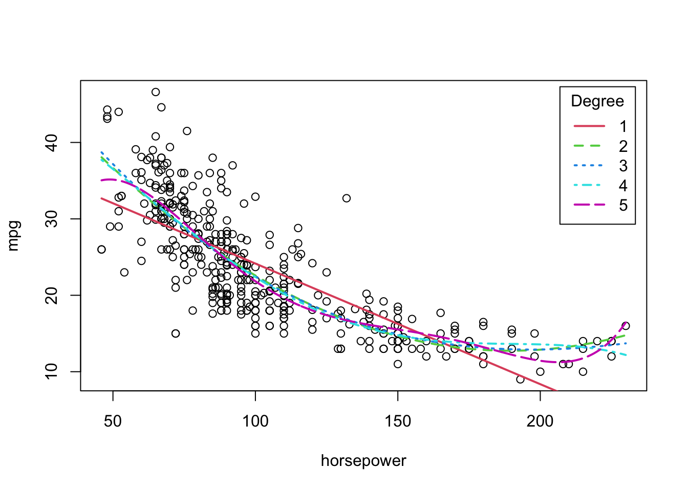
The relationship between the two variables is monotone, decreasing, and nonlinear. Following James et al. (2021), we’ll consider approximating the relationship by a polynomial regression, with the degree of the polynomial $p$ ranging from 1 (a linear regression) to 10.² Polynomial fits for $p = 1$ to $5$ are shown in the following figure:

plot(mpg ~ horsepower, data = Auto)
horsepower <- with(Auto,
                   seq(min(horsepower), max(horsepower),
                       length = 1000))
for (p in 1:5) {
  m <- lm(mpg ~ poly(horsepower, p), data = Auto)
  mpg <- predict(m, newdata = data.frame(horsepower = horsepower))
  lines(horsepower,
        mpg,
        col = p + 1,
        lty = p,
        lwd = 2)
}
legend(
  "topright",
  legend = 1:5,
  col = 2:6,
  lty = 1:5,
  lwd = 2,
  title = "Degree",
  inset = 0.02
)

mpg vs horsepower for the Auto data

The linear fit is clearly inappropriate; the fits for $p = 2$ (quadratic) through $4$ are very similar; and the fit for $p = 5$ may over-fit the data by chasing one or two relatively high mpg values at the right (but see the CV results reported below).

The following graph shows two measures of estimated (squared) error as a function of polynomial-regression degree: The mean-squared error (“MSE”), defined as $\mathsf{MSE} = \frac{1}{n}\sum_{i=1}^n (y_i - \widehat{y}_i)^2$, and the usual residual variance, defined as $\widehat{\sigma}^2 = \frac{1}{n - p - 1} \sum_{i=1}^n (y_i - \widehat{y}_i)^2$. The former necessarily declines with $p$ (or, more strictly, can’t increase with $p$), while the latter gets slightly larger for the largest values of $p$, with the “best” value, by a small margin, for $p = 7$.

library("cv") # for mse() and other functions
#> Loading required package: doParallel
#> Loading required package: foreach
#> Loading required package: iterators
#> Loading required package: parallel

var <- mse <- numeric(10)
for (p in 1:10) {
  m <- lm(mpg ~ poly(horsepower, p), data = Auto)
  mse[p] <- mse(Auto$mpg, fitted(m))
  var[p] <- summary(m)$sigma ^ 2
}

plot(
  c(1, 10),
  range(mse, var),
  type = "n",
  xlab = "Degree of polynomial, p",
  ylab = "Estimated Squared Error"
)
lines(
  1:10,
  mse,
  lwd = 2,
  lty = 1,
  col = 2,
  pch = 16,
  type = "b"
)
lines(
  1:10,
  var,
  lwd = 2,
  lty = 2,
  col = 3,
  pch = 17,
  type = "b"
)
legend(
  "topright",
  inset = 0.02,
  legend = c(expression(hat(sigma) ^ 2), "MSE"),
  lwd = 2,
  lty = 2:1,
  col = 3:2,
  pch = 17:16
)

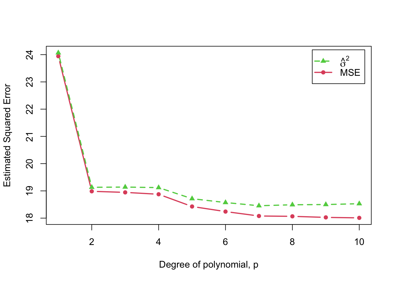
Estimated squared error as a function of polynomial degree, $p$

The code for this graph uses the mse() function from the cv package to compute the MSE for each fit.

Using cv()

The generic cv() function has an "lm" method, which by default performs $k = 10$-fold CV:

m.auto <- lm(mpg ~ poly(horsepower, 2), data = Auto)
summary(m.auto)
#> 
#> Call:
#> lm(formula = mpg ~ poly(horsepower, 2), data = Auto)
#> 
#> Residuals:
#>     Min      1Q  Median      3Q     Max 
#> -14.714  -2.594  -0.086   2.287  15.896 
#> 
#> Coefficients:
#>                      Estimate Std. Error t value Pr(>|t|)    
#> (Intercept)            23.446      0.221   106.1   <2e-16 ***
#> poly(horsepower, 2)1 -120.138      4.374   -27.5   <2e-16 ***
#> poly(horsepower, 2)2   44.090      4.374    10.1   <2e-16 ***
#> ---
#> Signif. codes:  0 '***' 0.001 '**' 0.01 '*' 0.05 '.' 0.1 ' ' 1
#> 
#> Residual standard error: 4.37 on 389 degrees of freedom
#> Multiple R-squared:  0.688,  Adjusted R-squared:  0.686 
#> F-statistic:  428 on 2 and 389 DF,  p-value: <2e-16

cv(m.auto)
#> R RNG seed set to 841111
#> cross-validation criterion (mse) = 19.25

The "lm" method by default uses mse() as the CV criterion and the Woodbury matrix identity (Hager, 1989) to update the regression with each fold deleted without having literally to refit the model. (Computational details are discussed in a separate vignette.) The print() method for "cv" objects simply print the cross-validation criterion, here the MSE. We can use summary() to obtain more information (as we’ll do routinely in the sequel):

summary(cv.m.auto <- cv(m.auto))
#> R RNG seed set to 411860
#> 10-Fold Cross Validation
#> method: Woodbury
#> criterion: mse
#> cross-validation criterion = 19.145
#> bias-adjusted cross-validation criterion = 19.136
#> full-sample criterion = 18.985

The summary reports the CV estimate of MSE, a biased-adjusted estimate of the MSE (the bias adjustment is explained in the final section), and the MSE is also computed for the original, full-sample regression. Because the division of the data into 10 folds is random, cv() explicitly (randomly) generates and saves a seed for R’s pseudo-random number generator, to make the results replicable. The user can also specify the seed directly via the seed argument to cv().

The plot() method for "cv" objects graphs the CV criterion (here MSE) by fold or the coefficients estimates with each fold deleted:

plot(cv.m.auto) # CV criterion

CV criterion (MSE) for cases in each fold.

plot(cv.m.auto, what="coefficients") # coefficient estimates

Regression coefficients with each fold omitted.

To perform LOO CV, we can set the k argument to cv() to the number of cases in the data, here k=392, or, more conveniently, to k="loo" or k="n":

summary(cv(m.auto, k = "loo"))
#> n-Fold Cross Validation
#> method: hatvalues
#> criterion: mse
#> cross-validation criterion = 19.248

For LOO CV of a linear model, cv() by default uses the hatvalues from the model fit to the full data for the LOO updates, and reports only the CV estimate of MSE. Alternative methods are to use the Woodbury matrix identity or the “naive” approach of literally refitting the model with each case omitted. All three methods produce exact results for a linear model (within the precision of floating-point computations):

summary(cv(m.auto, k = "loo", method = "naive"))
#> n-Fold Cross Validation
#> method: naive
#> criterion: mse
#> cross-validation criterion = 19.248
#> bias-adjusted cross-validation criterion = 19.248
#> full-sample criterion = 18.985

summary(cv(m.auto, k = "loo", method = "Woodbury"))
#> n-Fold Cross Validation
#> method: Woodbury
#> criterion: mse
#> cross-validation criterion = 19.248
#> bias-adjusted cross-validation criterion = 19.248
#> full-sample criterion = 18.985

The "naive" and "Woodbury" methods also return the bias-adjusted estimate of MSE and the full-sample MSE, but bias isn’t an issue for LOO CV.

Comparing competing models

The cv() function also has a method that can be applied to a list of regression models for the same data, composed using the models() function. For $k$-fold CV, the same folds are used for the competing models, which reduces random error in their comparison. This result can also be obtained by specifying a common seed for R’s random-number generator while applying cv() separately to each model, but employing a list of models is more convenient for both $k$-fold and LOO CV (where there is no random component to the composition of the $n$ folds).

We illustrate with the polynomial regression models of varying degree for the Auto data (discussed previously), beginning by fitting and saving the 10 models:

for (p in 1:10) {
  command <- paste0("m.", p, "<- lm(mpg ~ poly(horsepower, ", p,
                    "), data=Auto)")
  eval(parse(text = command))
}
objects(pattern = "m\\.[0-9]")
#>  [1] "m.1"  "m.10" "m.2"  "m.3"  "m.4"  "m.5"  "m.6"  "m.7"  "m.8"  "m.9"
summary(m.2) # for example, the quadratic fit
#> 
#> Call:
#> lm(formula = mpg ~ poly(horsepower, 2), data = Auto)
#> 
#> Residuals:
#>     Min      1Q  Median      3Q     Max 
#> -14.714  -2.594  -0.086   2.287  15.896 
#> 
#> Coefficients:
#>                      Estimate Std. Error t value Pr(>|t|)    
#> (Intercept)            23.446      0.221   106.1   <2e-16 ***
#> poly(horsepower, 2)1 -120.138      4.374   -27.5   <2e-16 ***
#> poly(horsepower, 2)2   44.090      4.374    10.1   <2e-16 ***
#> ---
#> Signif. codes:  0 '***' 0.001 '**' 0.01 '*' 0.05 '.' 0.1 ' ' 1
#> 
#> Residual standard error: 4.37 on 389 degrees of freedom
#> Multiple R-squared:  0.688,  Adjusted R-squared:  0.686 
#> F-statistic:  428 on 2 and 389 DF,  p-value: <2e-16

The convoluted code within the loop to produce the 10 models insures that the model formulas are of the form, e.g., mpg ~ poly(horsepower, 2) rather than mpg ~ poly(horsepower, p), which will be useful to us in a separate vignette, where we consider cross-validating the model-selection process.

We then apply cv() to the list of 10 models (the data argument is required):

# 10-fold CV
cv.auto.10 <- cv(
  models(m.1, m.2, m.3, m.4, m.5,
         m.6, m.7, m.8, m.9, m.10),
  data = Auto,
  seed = 2120
)
cv.auto.10[1:2] # for the linear and quadratic models
#> Model model.1:
#> cross-validation criterion = 24.246 
#> 
#> Model model.2:
#> cross-validation criterion = 19.346
summary(cv.auto.10)
#> 
#> Model model.1:
#> 10-Fold Cross Validation
#> method: Woodbury
#> cross-validation criterion = 24.246
#> bias-adjusted cross-validation criterion = 24.23
#> full-sample criterion = 23.944
#> 
#> Model model.2:
#> 10-Fold Cross Validation
#> method: Woodbury
#> cross-validation criterion = 19.346
#> bias-adjusted cross-validation criterion = 19.327
#> full-sample criterion = 18.985
#> 
#> Model model.3:
#> 10-Fold Cross Validation
#> method: Woodbury
#> cross-validation criterion = 19.396
#> bias-adjusted cross-validation criterion = 19.373
#> full-sample criterion = 18.945
#> 
#> Model model.4:
#> 10-Fold Cross Validation
#> method: Woodbury
#> cross-validation criterion = 19.444
#> bias-adjusted cross-validation criterion = 19.414
#> full-sample criterion = 18.876
#> 
#> Model model.5:
#> 10-Fold Cross Validation
#> method: Woodbury
#> cross-validation criterion = 19.014
#> bias-adjusted cross-validation criterion = 18.983
#> full-sample criterion = 18.427
#> 
#> Model model.6:
#> 10-Fold Cross Validation
#> method: Woodbury
#> cross-validation criterion = 18.954
#> bias-adjusted cross-validation criterion = 18.916
#> full-sample criterion = 18.241
#> 
#> Model model.7:
#> 10-Fold Cross Validation
#> method: Woodbury
#> cross-validation criterion = 18.898
#> bias-adjusted cross-validation criterion = 18.854
#> full-sample criterion = 18.078
#> 
#> Model model.8:
#> 10-Fold Cross Validation
#> method: Woodbury
#> cross-validation criterion = 19.126
#> bias-adjusted cross-validation criterion = 19.068
#> full-sample criterion = 18.066
#> 
#> Model model.9:
#> 10-Fold Cross Validation
#> method: Woodbury
#> cross-validation criterion = 19.342
#> bias-adjusted cross-validation criterion = 19.269
#> full-sample criterion = 18.027
#> 
#> Model model.10:
#> 10-Fold Cross Validation
#> method: Woodbury
#> cross-validation criterion = 20.012
#> bias-adjusted cross-validation criterion = 19.882
#> full-sample criterion = 18.01

# LOO CV
cv.auto.loo <- cv(models(m.1, m.2, m.3, m.4, m.5,
                         m.6, m.7, m.8, m.9, m.10),
                  data = Auto,
                  k = "loo")
cv.auto.loo[1:2] # linear and quadratic models
#> Model model.1:
#> cross-validation criterion = 24.232 
#> 
#> Model model.2:
#> cross-validation criterion = 19.248
summary(cv.auto.loo)
#> 
#> Model model.1:
#> n-Fold Cross Validation
#> method: hatvalues
#> cross-validation criterion = 24.232
#> 
#> Model model.2:
#> n-Fold Cross Validation
#> method: hatvalues
#> cross-validation criterion = 19.248
#> 
#> Model model.3:
#> n-Fold Cross Validation
#> method: hatvalues
#> cross-validation criterion = 19.335
#> 
#> Model model.4:
#> n-Fold Cross Validation
#> method: hatvalues
#> cross-validation criterion = 19.424
#> 
#> Model model.5:
#> n-Fold Cross Validation
#> method: hatvalues
#> cross-validation criterion = 19.033
#> 
#> Model model.6:
#> n-Fold Cross Validation
#> method: hatvalues
#> cross-validation criterion = 18.979
#> 
#> Model model.7:
#> n-Fold Cross Validation
#> method: hatvalues
#> cross-validation criterion = 18.833
#> 
#> Model model.8:
#> n-Fold Cross Validation
#> method: hatvalues
#> cross-validation criterion = 18.961
#> 
#> Model model.9:
#> n-Fold Cross Validation
#> method: hatvalues
#> cross-validation criterion = 19.069
#> 
#> Model model.10:
#> n-Fold Cross Validation
#> method: hatvalues
#> cross-validation criterion = 19.491

Because we didn’t supply names for the models in the calls to the models() function, the names model.1, model.2, etc., are generated by the function.

Finally, we extract and graph the adjusted MSEs for $10$-fold CV and the MSEs for LOO CV (see the section below on manipulating "cv" objects:

cv.mse.10 <- as.data.frame(cv.auto.10, 
                           rows="cv",             
                           columns="criteria"
                           )$adjusted.criterion
cv.mse.loo <- as.data.frame(cv.auto.loo, 
                           rows="cv",             
                           columns="criteria"
                           )$criterion
plot(
  c(1, 10),
  range(cv.mse.10, cv.mse.loo),
  type = "n",
  xlab = "Degree of polynomial, p",
  ylab = "Cross-Validated MSE"
)
lines(
  1:10,
  cv.mse.10,
  lwd = 2,
  lty = 1,
  col = 2,
  pch = 16,
  type = "b"
)
lines(
  1:10,
  cv.mse.loo,
  lwd = 2,
  lty = 2,
  col = 3,
  pch = 17,
  type = "b"
)
legend(
  "topright",
  inset = 0.02,
  legend = c("10-Fold CV", "LOO CV"),
  lwd = 2,
  lty = 2:1,
  col = 3:2,
  pch = 17:16
)

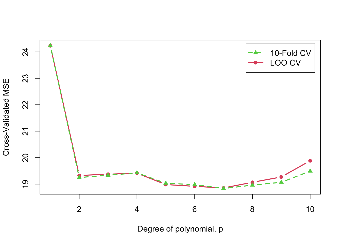
Cross-validated 10-fold and LOO MSE as a function of polynomial degree, $p$

Alternatively, we can use the plot() method for "cvModList" objects to compare the models, though with separate graphs for 10-fold and LOO CV:

plot(cv.auto.10, main="Polynomial Regressions, 10-Fold CV",
     axis.args=list(labels=1:10), xlab="Degree of Polynomial, p")
plot(cv.auto.loo, main="Polynomial Regressions, LOO CV",
     axis.args=list(labels=1:10), xlab="Degree of Polynomial, p")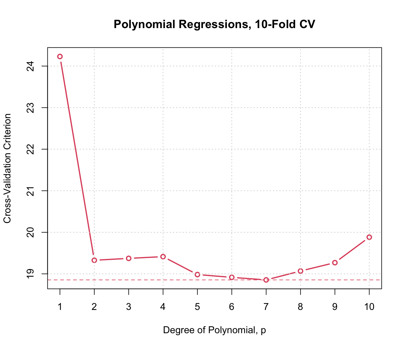

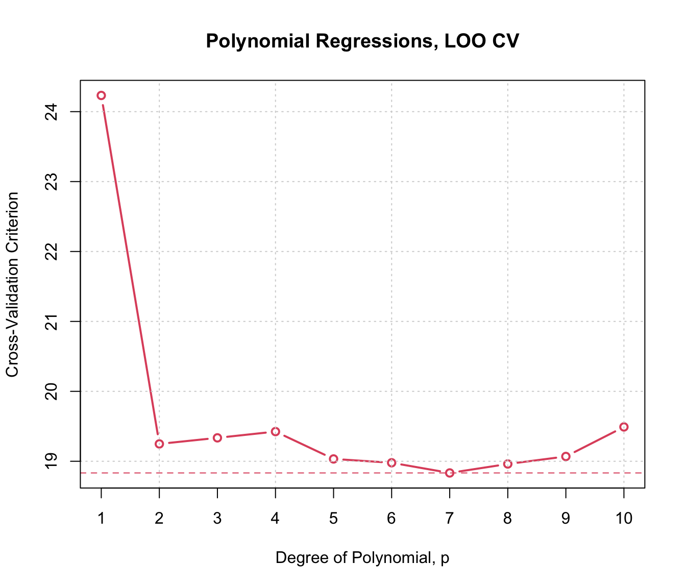
Cross-validated 10-fold and LOO MSE as a function of polynomial degree, $p$

In this example, 10-fold and LOO CV produce generally similar results, and also results that are similar to those produced by the estimated error variance $\widehat{\sigma}^2$ for each model, reported above (except for the highest-degree polynomials, where the CV results more clearly suggest over-fitting).

Logistic regression for the Mroz data

The Mroz data set from the carData package (associated with Fox & Weisberg, 2019) has been used by several authors to illustrate binary logistic regression; see, in particular Fox & Weisberg (2019). The data were originally drawn from the U.S. Panel Study of Income Dynamics and pertain to married women. Here are a few cases in the data set:

data("Mroz", package = "carData")
head(Mroz, 3)
#>   lfp k5 k618 age wc hc    lwg   inc
#> 1 yes  1    0  32 no no 1.2102 10.91
#> 2 yes  0    2  30 no no 0.3285 19.50
#> 3 yes  1    3  35 no no 1.5141 12.04
tail(Mroz, 3)
#>     lfp k5 k618 age wc hc     lwg    inc
#> 751  no  0    0  43 no no 0.88814  9.952
#> 752  no  0    0  60 no no 1.22497 24.984
#> 753  no  0    3  39 no no 0.85321 28.363

The response variable in the logistic regression is lfp, labor-force participation, a factor coded "yes" or "no". The remaining variables are predictors:

• k5, number of children 5 years old of younger in the woman’s household;
• k618, number of children between 6 and 18 years old;
• age, in years;
• wc, wife’s college attendance, "yes" or "no";
• hc, husband’s college attendance;
• lwg, the woman’s log wage rate if she is employed, or her imputed wage rate, if she is not (a variable that Fox & Weisberg, 2019 show is problematically defined); and
• inc, family income, in $1000s, exclusive of wife’s income.

We use the glm() function to fit a binary logistic regression to the Mroz data:

m.mroz <- glm(lfp ~ ., data = Mroz, family = binomial)
summary(m.mroz)
#> 
#> Call:
#> glm(formula = lfp ~ ., family = binomial, data = Mroz)
#> 
#> Coefficients:
#>             Estimate Std. Error z value Pr(>|z|)    
#> (Intercept)  3.18214    0.64438    4.94  7.9e-07 ***
#> k5          -1.46291    0.19700   -7.43  1.1e-13 ***
#> k618        -0.06457    0.06800   -0.95  0.34234    
#> age         -0.06287    0.01278   -4.92  8.7e-07 ***
#> wcyes        0.80727    0.22998    3.51  0.00045 ***
#> hcyes        0.11173    0.20604    0.54  0.58762    
#> lwg          0.60469    0.15082    4.01  6.1e-05 ***
#> inc         -0.03445    0.00821   -4.20  2.7e-05 ***
#> ---
#> Signif. codes:  0 '***' 0.001 '**' 0.01 '*' 0.05 '.' 0.1 ' ' 1
#> 
#> (Dispersion parameter for binomial family taken to be 1)
#> 
#>     Null deviance: 1029.75  on 752  degrees of freedom
#> Residual deviance:  905.27  on 745  degrees of freedom
#> AIC: 921.3
#> 
#> Number of Fisher Scoring iterations: 4

BayesRule(ifelse(Mroz$lfp == "yes", 1, 0),
          fitted(m.mroz, type = "response"))
#> [1] 0.30677
#> attr(,"casewise loss")
#> [1] "y != round(yhat)"

In addition to the usually summary output for a GLM, we show the result of applying the BayesRule() function from the cv package to predictions derived from the fitted model. Bayes rule, which predicts a “success” in a binary regression model when the fitted probability of success [i.e., $\phi = \Pr(y = 1)$] is $\widehat{\phi} \ge .5$ and a “failure” if $\widehat{\phi} \lt .5$.³ The first argument to BayesRule() is the binary {0, 1} response, and the second argument is the predicted probability of success. BayesRule() returns the proportion of predictions that are in error, as appropriate for a “cost” function.

The value returned by BayesRule() is associated with an “attribute” named "casewise loss" and set to "y != round(yhat)", signifying that the Bayes rule CV criterion is computed as the mean of casewise values, here 0 if the prediction for a case matches the observed value and 1 if it does not (signifying a prediction error). The mse() function for numeric responses is also calculated as a casewise average. Some other criteria, such as the median absolute error, computed by the medAbsErr() function in the cv package, aren’t averages of casewise components. The distinction is important because, to our knowledge, the statistical theory of cross-validation, for example, in Davison & Hinkley (1997), Bates, Hastie, & Tibshirani (2023), and Arlot & Celisse (2010), is developed for CV criteria like MSE that are means of casewise components. As a consequence, we limit computation of bias adjustment and confidence intervals (see below) to criteria that are casewise averages.

In this example, the fitted logistic regression incorrectly predicts 31% of the responses; we expect this estimate to be optimistic given that the model is used to “predict” the data to which it is fit.

The "glm" method for cv() is largely similar to the "lm" method, although the default algorithm, selected explicitly by method="exact", refits the model with each fold removed (and is thus equivalent to method="naive" for "lm" models). For generalized linear models, method="Woodbury" or (for LOO CV) method="hatvalues" provide approximate results (see the computational and technical vignette for details):

summary(cv(m.mroz, criterion = BayesRule, seed = 248))
#> R RNG seed set to 248
#> 10-Fold Cross Validation
#> method: exact
#> criterion: BayesRule
#> cross-validation criterion = 0.32404
#> bias-adjusted cross-validation criterion = 0.31952
#> 95% CI for bias-adjusted CV criterion = (0.28607, 0.35297)
#> full-sample criterion = 0.30677

summary(cv(m.mroz,
   criterion = BayesRule,
   seed = 248,
   method = "Woodbury"))
#> R RNG seed set to 248
#> 10-Fold Cross Validation
#> method: Woodbury
#> criterion: BayesRule
#> cross-validation criterion = 0.32404
#> bias-adjusted cross-validation criterion = 0.31926
#> 95% CI for bias-adjusted CV criterion = (0.28581, 0.35271)
#> full-sample criterion = 0.30677

To ensure that the two methods use the same 10 folds, we specify the seed for R’s random-number generator explicitly; here, and as is common in our experience, the "exact" and "Woodbury" algorithms produce nearly identical results. The CV estimates of prediction error are slightly higher than the estimate based on all of the cases.

The printed output includes a 95% confidence interval for the bias-adjusted Bayes rule CV criterion. Bates et al. (2023) show that these confidence intervals are unreliable for models fit to small samples, and by default cv() computes them only when the sample size is 400 or larger and when the CV criterion employed is an average of casewise components, as is the case for Bayes rule. See the final section of the vignette for details of the computation of confidence intervals for bias-adjusted CV criteria.

Here are results of applying LOO CV to the Mroz model, using both the exact and the approximate methods:

summary(cv(m.mroz, k = "loo", criterion = BayesRule))
#> n-Fold Cross Validation
#> method: exact
#> criterion: BayesRule
#> cross-validation criterion = 0.32005
#> bias-adjusted cross-validation criterion = 0.3183
#> 95% CI for bias-adjusted CV criterion = (0.28496, 0.35164)
#> full-sample criterion = 0.30677

summary(cv(m.mroz,
   k = "loo",
   criterion = BayesRule,
   method = "Woodbury"))
#> n-Fold Cross Validation
#> method: Woodbury
#> criterion: BayesRule
#> cross-validation criterion = 0.32005
#> bias-adjusted cross-validation criterion = 0.3183
#> 95% CI for bias-adjusted CV criterion = (0.28496, 0.35164)
#> full-sample criterion = 0.30677

summary(cv(m.mroz,
   k = "loo",
   criterion = BayesRule,
   method = "hatvalues"))
#> n-Fold Cross Validation
#> method: hatvalues
#> criterion: BayesRule
#> cross-validation criterion = 0.32005

To the number of decimal digits shown, the three methods produce identical results for this example.

Replicating cross-validation

Assuming that the number of cases $n$ is a multiple of the number of folds $k$—a slightly simplifying assumption—the number of possible partitions of cases into folds is $\frac{n!}{[(n/k)!]^k}$, a number that grows very large very quickly. For example, for $n = 10$ and $k = 5$, so that the folds are each of size $n/k = 2$, there are $113,400$ possible partitions; for $n=100$ and $k=5$, where $n/k = 20$, still a small problem, the number of possible partitions is truly astronomical, $1.09\times 10^{66}$.

Because the partition into folds that’s employed is selected randomly, the resulting CV criterion estimates are subject to sampling error. (An exception is LOO cross-validation, which is not at all random.) To get a sense of the magnitude of the sampling error, we can repeat the CV procedure with different randomly selected partitions into folds. All of the CV functions in the cv package are capable of repeated cross-validation, with the number of repetitions controlled by the reps argument, which defaults to 1.

Here, for example, is 10-fold CV for the Mroz logistic regression, repeated 5 times:

summary(cv.mroz.reps <- cv(
  m.mroz,
  criterion = BayesRule,
  seed = 248,
  reps = 5,
  method = "Woodbury"
))
#> R RNG seed set to 248
#> R RNG seed set to 68134
#> R RNG seed set to 767359
#> R RNG seed set to 556270
#> R RNG seed set to 882966
#> 
#> Replicate 1:
#> 10-Fold Cross Validation
#> method: Woodbury
#> criterion: BayesRule
#> cross-validation criterion = 0.32005
#> bias-adjusted cross-validation criterion = 0.31301
#> 95% CI for bias-adjusted CV criterion = (0.27967, 0.34635)
#> full-sample criterion = 0.30677
#> 
#> Replicate 2:
#> 10-Fold Cross Validation
#> method: Woodbury
#> criterion: BayesRule
#> cross-validation criterion = 0.31607
#> bias-adjusted cross-validation criterion = 0.3117
#> 95% CI for bias-adjusted CV criterion = (0.27847, 0.34493)
#> full-sample criterion = 0.30677
#> 
#> Replicate 3:
#> 10-Fold Cross Validation
#> method: Woodbury
#> criterion: BayesRule
#> cross-validation criterion = 0.31474
#> bias-adjusted cross-validation criterion = 0.30862
#> 95% CI for bias-adjusted CV criterion = (0.27543, 0.34181)
#> full-sample criterion = 0.30677
#> 
#> Replicate 4:
#> 10-Fold Cross Validation
#> method: Woodbury
#> criterion: BayesRule
#> cross-validation criterion = 0.32404
#> bias-adjusted cross-validation criterion = 0.31807
#> 95% CI for bias-adjusted CV criterion = (0.28462, 0.35152)
#> full-sample criterion = 0.30677
#> 
#> Replicate 5:
#> 10-Fold Cross Validation
#> method: Woodbury
#> criterion: BayesRule
#> cross-validation criterion = 0.32404
#> bias-adjusted cross-validation criterion = 0.31926
#> 95% CI for bias-adjusted CV criterion = (0.28581, 0.35271)
#> full-sample criterion = 0.30677
#> 
#> Average:
#> 10-Fold Cross Validation
#> method: Woodbury
#> criterion: BayesRule
#> cross-validation criterion = 0.31983 (0.003887)
#> bias-adjusted cross-validation criterion = 0.31394 (0.0040093)
#> full-sample criterion = 0.30677

When reps > 1, the result returned by cv() is an object of class "cvList"—literally a list of "cv" objects. The results are reported for each repetition and then averaged across repetitions, with the standard deviations of the CV criterion and the biased-adjusted CV criterion given in parentheses. In this example, there is therefore little variation across repetitions, increasing our confidence in the reliability of the results.

Notice that the seed that’s set in the cv() command pertains to the first repetition and the seeds for the remaining repetitions are then selected pseudo-randomly.⁴ Setting the first seed, however, makes the entire process easily replicable, and the seed for each repetition is stored in the corresponding element of the "cvList" object.

The plot() method for "cvList" objects by default shows the adjusted CV criterion and confidence interval for each replication:

plot(cv.mroz.reps)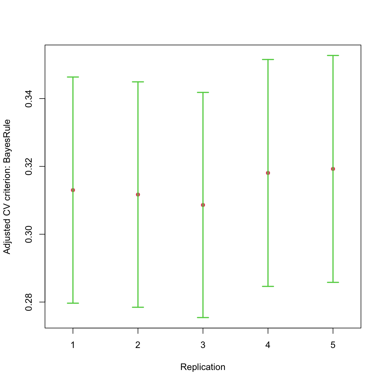

Replicated cross-validated 10-fold CV for the logistic regression fit to the Mroz data.

It’s also possible to replicate CV when comparing competing models via the cv() method for "modList" objects. Recall our comparison of polynomial regressions of varying degree fit to the Auto data; we performed 10-fold CV for each of 10 models. Here, we replicate that process 5 times for each model and graph the results:

cv.auto.reps <- cv(
  models(m.1, m.2, m.3, m.4, m.5,
         m.6, m.7, m.8, m.9, m.10),
  data = Auto,
  seed = 8004,
  reps = 5
)
plot(cv.auto.reps)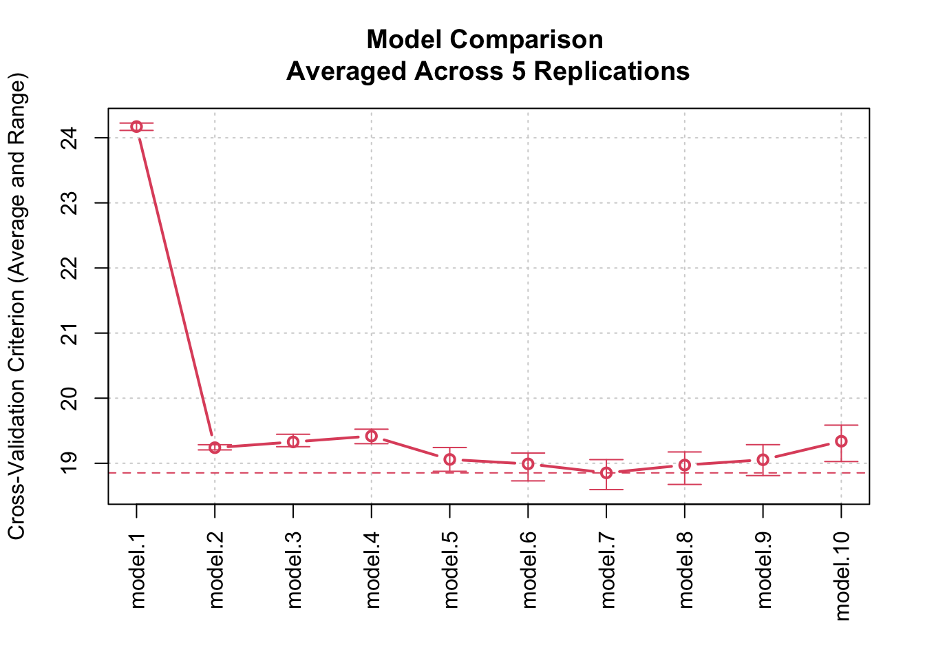

Replicated cross-validated 10-fold CV as a function of polynomial degree, $p$

The graph shows both the average CV criterion and its range for each of the competing models.

Manipulating “cv” and related objects

The cv() functions returns an object of class "cv"—or a closely related object, for example, of class "cvList"—which contains a variety of information about the results of a CV procedure. The cv package provides as.data.frame() methods to put this information in the form of data frames for further examination and analysis.⁵ There is also a summary() method for extracting and summarizing the information in the resulting data frames.

We’ll illustrate with the replicated CV that we performed for the 10 polynomial-regression models fit to the Auto data:

cv.auto.reps
#> Model model.1 averaged across 5 replications:
#> cross-validation criterion = 24.185 
#> 
#> Model model.2 averaged across 5 replications:
#> cross-validation criterion = 19.253 
#> 
#> Model model.3 averaged across 5 replications:
#> cross-validation criterion = 19.349 
#> 
#> Model model.4 averaged across 5 replications:
#> cross-validation criterion = 19.449 
#> 
#> Model model.5 averaged across 5 replications:
#> cross-validation criterion = 19.095 
#> 
#> Model model.6 averaged across 5 replications:
#> cross-validation criterion = 19.034 
#> 
#> Model model.7 averaged across 5 replications:
#> cross-validation criterion = 18.897 
#> 
#> Model model.8 averaged across 5 replications:
#> cross-validation criterion = 19.026 
#> 
#> Model model.9 averaged across 5 replications:
#> cross-validation criterion = 19.115 
#> 
#> Model model.10 averaged across 5 replications:
#> cross-validation criterion = 19.427
class(cv.auto.reps)
#> [1] "cvModList"

In this case, there are 5 replications of 10-fold CV.

Converting cv.auto.reps into a data frame produces, by default:

D <- as.data.frame(cv.auto.reps)
dim(D)
#> [1] 550  62
class(D)
#> [1] "cvModListDataFrame" "cvListDataFrame"    "cvDataFrame"       
#> [4] "data.frame"

The resulting data frame has $\mathsf{replications} \times (\mathsf{folds} + 1) \times \mathsf{models} = 5 \times (10 + 1) \times 10 = 550$ rows, the first few of which are

head(D)
#>     model rep fold criterion adjusted.criterion full.criterion coef.Intercept
#> 1 model.1   1    0      24.2               24.2           23.9           23.4
#> 2 model.1   1    1      34.3                 NA             NA           23.3
#> 3 model.1   1    2      24.5                 NA             NA           23.3
#> 4 model.1   1    3      13.9                 NA             NA           23.6
#> 5 model.1   1    4      15.5                 NA             NA           23.5
#> 6 model.1   1    5      28.6                 NA             NA           23.4
#>   coef.poly(horsepower, 1) coef.poly(horsepower, 2)1 coef.poly(horsepower, 2)2
#> 1                     -120                        NA                        NA
#> 2                     -121                        NA                        NA
#> 3                     -119                        NA                        NA
#> 4                     -120                        NA                        NA
#> 5                     -118                        NA                        NA
#> 6                     -119                        NA                        NA
#>   coef.poly(horsepower, 3)1 coef.poly(horsepower, 3)2 coef.poly(horsepower, 3)3
#> 1                        NA                        NA                        NA
#> 2                        NA                        NA                        NA
#> 3                        NA                        NA                        NA
#> 4                        NA                        NA                        NA
#> 5                        NA                        NA                        NA
#> 6                        NA                        NA                        NA
#>   coef.poly(horsepower, 4)1 coef.poly(horsepower, 4)2 coef.poly(horsepower, 4)3
#> 1                        NA                        NA                        NA
#> 2                        NA                        NA                        NA
#> 3                        NA                        NA                        NA
#> 4                        NA                        NA                        NA
#> 5                        NA                        NA                        NA
#> 6                        NA                        NA                        NA
#>   coef.poly(horsepower, 4)4 coef.poly(horsepower, 5)1 coef.poly(horsepower, 5)2
#> 1                        NA                        NA                        NA
#> 2                        NA                        NA                        NA
#> 3                        NA                        NA                        NA
#> 4                        NA                        NA                        NA
#> 5                        NA                        NA                        NA
#> 6                        NA                        NA                        NA
#>   coef.poly(horsepower, 5)3 coef.poly(horsepower, 5)4 coef.poly(horsepower, 5)5
#> 1                        NA                        NA                        NA
#> 2                        NA                        NA                        NA
#> 3                        NA                        NA                        NA
#> 4                        NA                        NA                        NA
#> 5                        NA                        NA                        NA
#> 6                        NA                        NA                        NA
#>   coef.poly(horsepower, 6)1 coef.poly(horsepower, 6)2 coef.poly(horsepower, 6)3
#> 1                        NA                        NA                        NA
#> 2                        NA                        NA                        NA
#> 3                        NA                        NA                        NA
#> 4                        NA                        NA                        NA
#> 5                        NA                        NA                        NA
#> 6                        NA                        NA                        NA
#>   coef.poly(horsepower, 6)4 coef.poly(horsepower, 6)5 coef.poly(horsepower, 6)6
#> 1                        NA                        NA                        NA
#> 2                        NA                        NA                        NA
#> 3                        NA                        NA                        NA
#> 4                        NA                        NA                        NA
#> 5                        NA                        NA                        NA
#> 6                        NA                        NA                        NA
#>   coef.poly(horsepower, 7)1 coef.poly(horsepower, 7)2 coef.poly(horsepower, 7)3
#> 1                        NA                        NA                        NA
#> 2                        NA                        NA                        NA
#> 3                        NA                        NA                        NA
#> 4                        NA                        NA                        NA
#> 5                        NA                        NA                        NA
#> 6                        NA                        NA                        NA
#>   coef.poly(horsepower, 7)4 coef.poly(horsepower, 7)5 coef.poly(horsepower, 7)6
#> 1                        NA                        NA                        NA
#> 2                        NA                        NA                        NA
#> 3                        NA                        NA                        NA
#> 4                        NA                        NA                        NA
#> 5                        NA                        NA                        NA
#> 6                        NA                        NA                        NA
#>   coef.poly(horsepower, 7)7 coef.poly(horsepower, 8)1 coef.poly(horsepower, 8)2
#> 1                        NA                        NA                        NA
#> 2                        NA                        NA                        NA
#> 3                        NA                        NA                        NA
#> 4                        NA                        NA                        NA
#> 5                        NA                        NA                        NA
#> 6                        NA                        NA                        NA
#>   coef.poly(horsepower, 8)3 coef.poly(horsepower, 8)4 coef.poly(horsepower, 8)5
#> 1                        NA                        NA                        NA
#> 2                        NA                        NA                        NA
#> 3                        NA                        NA                        NA
#> 4                        NA                        NA                        NA
#> 5                        NA                        NA                        NA
#> 6                        NA                        NA                        NA
#>   coef.poly(horsepower, 8)6 coef.poly(horsepower, 8)7 coef.poly(horsepower, 8)8
#> 1                        NA                        NA                        NA
#> 2                        NA                        NA                        NA
#> 3                        NA                        NA                        NA
#> 4                        NA                        NA                        NA
#> 5                        NA                        NA                        NA
#> 6                        NA                        NA                        NA
#>   coef.poly(horsepower, 9)1 coef.poly(horsepower, 9)2 coef.poly(horsepower, 9)3
#> 1                        NA                        NA                        NA
#> 2                        NA                        NA                        NA
#> 3                        NA                        NA                        NA
#> 4                        NA                        NA                        NA
#> 5                        NA                        NA                        NA
#> 6                        NA                        NA                        NA
#>   coef.poly(horsepower, 9)4 coef.poly(horsepower, 9)5 coef.poly(horsepower, 9)6
#> 1                        NA                        NA                        NA
#> 2                        NA                        NA                        NA
#> 3                        NA                        NA                        NA
#> 4                        NA                        NA                        NA
#> 5                        NA                        NA                        NA
#> 6                        NA                        NA                        NA
#>   coef.poly(horsepower, 9)7 coef.poly(horsepower, 9)8 coef.poly(horsepower, 9)9
#> 1                        NA                        NA                        NA
#> 2                        NA                        NA                        NA
#> 3                        NA                        NA                        NA
#> 4                        NA                        NA                        NA
#> 5                        NA                        NA                        NA
#> 6                        NA                        NA                        NA
#>   coef.poly(horsepower, 10)1 coef.poly(horsepower, 10)2
#> 1                         NA                         NA
#> 2                         NA                         NA
#> 3                         NA                         NA
#> 4                         NA                         NA
#> 5                         NA                         NA
#> 6                         NA                         NA
#>   coef.poly(horsepower, 10)3 coef.poly(horsepower, 10)4
#> 1                         NA                         NA
#> 2                         NA                         NA
#> 3                         NA                         NA
#> 4                         NA                         NA
#> 5                         NA                         NA
#> 6                         NA                         NA
#>   coef.poly(horsepower, 10)5 coef.poly(horsepower, 10)6
#> 1                         NA                         NA
#> 2                         NA                         NA
#> 3                         NA                         NA
#> 4                         NA                         NA
#> 5                         NA                         NA
#> 6                         NA                         NA
#>   coef.poly(horsepower, 10)7 coef.poly(horsepower, 10)8
#> 1                         NA                         NA
#> 2                         NA                         NA
#> 3                         NA                         NA
#> 4                         NA                         NA
#> 5                         NA                         NA
#> 6                         NA                         NA
#>   coef.poly(horsepower, 10)9 coef.poly(horsepower, 10)10
#> 1                         NA                          NA
#> 2                         NA                          NA
#> 3                         NA                          NA
#> 4                         NA                          NA
#> 5                         NA                          NA
#> 6                         NA                          NA

All of these rows pertain to the first model and the first replication, and fold = 0 indicates the overall results for the first replication of the first model.

The regression coefficients appear as columns in the data frame. Because the first model includes only an intercept and a linear polynomial term, the other coefficients are all NA.

It’s possible to suppress the regression coefficients by specifying the argument columns="criteria" to as.data.frame():

D <- as.data.frame(cv.auto.reps, columns="criteria")
head(D)
#>     model rep fold criterion adjusted.criterion full.criterion
#> 1 model.1   1    0      24.2               24.2           23.9
#> 2 model.1   1    1      34.3                 NA             NA
#> 3 model.1   1    2      24.5                 NA             NA
#> 4 model.1   1    3      13.9                 NA             NA
#> 5 model.1   1    4      15.5                 NA             NA
#> 6 model.1   1    5      28.6                 NA             NA
head(subset(D, fold == 0))
#>      model rep fold criterion adjusted.criterion full.criterion
#> 1  model.1   1    0      24.2               24.2           23.9
#> 12 model.1   2    0      24.1               24.1           23.9
#> 23 model.1   3    0      24.2               24.2           23.9
#> 34 model.1   4    0      24.2               24.1           23.9
#> 45 model.1   5    0      24.2               24.2           23.9
#> 56 model.2   1    0      19.2               19.2           19.0

The summary() method for "cvDataFrame" and related objects has a formula interface, and may be used, for example, as follows:

summary(D, adjusted.criterion ~ model + rep) # fold "0" only
#>           rep
#> model           1      2      3      4      5
#>   model.1  24.193 24.113 24.226 24.144 24.184
#>   model.2  19.209 19.285 19.240 19.205 19.256
#>   model.3  19.309 19.445 19.348 19.255 19.282
#>   model.4  19.521 19.524 19.402 19.343 19.301
#>   model.5  19.242 19.139 19.137 18.877 18.899
#>   model.6  19.157 19.145 19.082 18.730 18.838
#>   model.7  18.935 19.056 18.960 18.596 18.715
#>   model.8  19.043 19.174 19.111 18.675 18.861
#>   model.9  19.133 19.286 19.161 18.811 18.880
#>   model.10 19.524 19.586 19.345 19.027 19.214
summary(D, criterion ~ model + rep, 
        include="folds") # mean over folds
#>           rep
#> model           1      2      3      4      5
#>   model.1  24.181 24.128 24.226 24.134 24.229
#>   model.2  19.202 19.310 19.236 19.193 19.306
#>   model.3  19.309 19.483 19.352 19.247 19.336
#>   model.4  19.536 19.571 19.415 19.342 19.360
#>   model.5  19.262 19.195 19.163 18.874 18.963
#>   model.6  19.182 19.217 19.116 18.731 18.910
#>   model.7  18.954 19.135 18.997 18.601 18.787
#>   model.8  19.071 19.259 19.162 18.686 18.944
#>   model.9  19.171 19.379 19.214 18.834 18.965
#>   model.10 19.603 19.710 19.416 19.068 19.329
summary(D, criterion ~ model + rep, fun=sd, 
        include="folds")
#>           rep
#> model           1      2      3      4      5
#>   model.1  7.5627 5.2658 5.7947 4.7165 7.3591
#>   model.2  5.9324 5.2518 5.8166 5.1730 6.2126
#>   model.3  6.0754 5.4492 5.8168 5.2288 6.2387
#>   model.4  6.1737 5.2488 5.9952 5.4866 6.3122
#>   model.5  5.7598 5.2136 6.2658 5.3923 6.3016
#>   model.6  5.7094 5.0444 6.4010 5.2868 5.9796
#>   model.7  5.6307 5.1164 6.6751 5.1084 5.8796
#>   model.8  5.7009 5.1229 6.4827 5.1068 5.9460
#>   model.9  5.7979 5.2289 6.3960 5.3181 6.0902
#>   model.10 6.1825 4.8554 6.2557 5.7029 6.1985

See ?summary.cvDataFrame for details.

Parallel computations

The CV functions in the cv package are all capable of performing parallel computations by setting the ncores argument (specifying the number of computer cores to be used) to a number > 1 (which is the default). Parallel computation can be advantageous for large problems, reducing the execution time of the program.

To illustrate, let’s time model selection in Mroz’s logistic regression, repeating the computation as performed previously (but with LOO CV to lengthen the calculation) and then doing it in parallel using 2 cores:

system.time(
  m.mroz.sel.cv <- cv(
    selectStepAIC,
    Mroz,
    k = "loo",
    criterion = BayesRule,
    working.model = m.mroz,
    AIC = FALSE
  )
)
#>    user  system elapsed 
#>  22.644   0.482  23.145

system.time(
  m.mroz.sel.cv.p <- cv(
    selectStepAIC,
    Mroz,
    k = "loo",
    criterion = BayesRule,
    working.model = m.mroz,
    AIC = FALSE,
    ncores = 2
  )
)
#>    user  system elapsed 
#>   0.228   0.045  14.396
all.equal(m.mroz.sel.cv, m.mroz.sel.cv.p)
#> [1] TRUE

On our computer, the parallel computation with 2 cores is nearly twice as fast, and produces the same result as the non-parallel computation.

References

Arlot, S., & Celisse, A. (2010). A survey of cross-validation procedures for model selection. Statistics Surveys, 4, 40–79. Retrieved from https://doi.org/10.1214/09-SS054

Bates, S., Hastie, T., & Tibshirani, R. (2023). Cross-validation: What does it estimate and how well does it do it? Journal of the American Statistical Association, in press. Retrieved from https://doi.org/10.1080/01621459.2023.2197686

Canty, A., & Ripley, B. D. (2022). Boot: Bootstrap R (S-plus) functions.

Davison, A. C., & Hinkley, D. V. (1997). Bootstrap methods and their applications. Cambridge: Cambridge University Press.

Fox, J., & Weisberg, S. (2019). An R companion to applied regression (Third edition). Thousand Oaks CA: Sage.

Hager, W. W. (1989). Updating the inverse of a matrix. SIAM Review, 31(2), 221–239.

Harrell, F., Jr. (2015). Regression modeling strategies (Second edition). New York: Springer.

James, G., Witten, D., Hastie, T., & Tibshirani, R. (2021). An introduction to statistical learning with applications in R (Second edition). New York: Springer.